The art of growth and the solution of cognitive problems

Philip Van Loocke

Lab for Applied Epistemology, University of Ghent, Belgium

e-mail: philip.vanloocke@rug.ac.be

 

 

Abstract

A cellular method is proposed as an alternative for a connectionist approach. The present method does not use connections between cells, but introduces a field concept instead. If the fields are determined in accordance with the transformations familiar from fractal theory, then the solutions of problems that have some symmetry are forms of remarkable beauty. This way, a link is proposed between generative art and problem solving. It is conjectured that the ‘black box’ nature of connectionist systems can be replaced by an approach in which the solution of a problem coincides with a vivid visualization, also if the problems at hand are of a high-dimensional nature.

1. Introduction

The world is full of problems. Since Leibniz, the ideal of many scientists was to cast them in a mathematical form. Then, calculus would bring forward solutions agreed upon by every fellow scientist. As has been argued by Yates (1966), this part of Leibniz’ philosophy is a modernist translation of older renaissance and medieval ideas, connected mainly with Ramon Lull. Lull defended that every part of the cosmos could be contemplated by allowing symbols to mentally rotate on concentric wheels. The symbol combinations that result would correspond to the properties and entities of God’s creature.

 

But Lull was not typical for his time. The typical consciousness of the philosopher of the middle ages was not a consciousness in which symbols were contemplated, but a consciousness in which vivid imagery was prolific. According to Yates’ thesis, this imagery was related to the fact that books were much more precious, so that memorizing items or lines of argument was more important than it is now. As was well known, vivid imagery significantly helps memory. The ‘art’ of memory was carefully elaborated by many authors, such as Albertus Magnus, Romberch, Rosellius, and so on. It can be conjectured that this art had a profound influence on medieval and renaissance philosophy. However, a vivid imagery accords with a general medieval mentality, not restricted to intellectual elite groups, in which a vivid imagination of Gods punishments and rewards was instrumental for the maintenance of moral order in society. Further, it agrees with the medieval attitude in which thinking was dominated much more by analogy, and by reference to abounding proverbs, instead of by analysis of situations in causal terms (Huizinga, 1954).

 

Bruno took advantage of Ramon Lull’s scheme for mental rotation in order to reform the medieval imageristic states typical for contemplating philosophers. In Bruno’s ‘art’, the images in one’s imagination had to rotate on concentric wheels. This way, a theatre was created in consciousness, and the devote person had to let the theatre play (by rotating the wheels) in order to mirror in his consciousness all parts and all levels of the cosmos. However, Bruno’s synthesis of Lull and renaissance imagery was a swan song. Not only did it refer too much to renaissance magic (for which he was burned). The iconoclastic fury of the puritan protestant movement antagonized with the imageristic approach to knowledge. But most of all, a rationalized version of Lull’s symbol manipulation approach would become canonical with the advent of modern science. Even though it may be argued that modern science may not have emerged at all without its renaissance and medieval antecedents, it cut away the vivid imageristic part of the consciousness of the knowing subject, which was so typical for these ages. In our days, at most some schematic imagery may enter consciousness when theoretical science is performed. Bruno would not understand that people want to do science if this means that their consciousness is so monotonic and pale.

 

Since the advent of the computer and of the complexity sciences, some problems in science became associated with nice images again. However, the most aesthetic fractal, the Mandelbrot set, has no application outside theoretical mathematics at the moment. In cognitive science, the aesthetics of fractals has does far not penetrated at all. Here, we show how aesthetics can be introduced in problem solving in general. It takes a reformulation of connectionism, in which connections are replaced by fields. Also, it requires the insertion of some elementary concepts from the domain of fractals in the definition of these fields. Obviously, medieval or renaissance problem solving imagery will never come back. But nevertheless, one may conjecture that generative art and problem solving can be linked in a natural way.

 

2. Connections and fields in cellular systems

A connectionist system, or neural network, operates on basis of simple neural processors and connections. The latter determine the internal communication in a network. In case of a Hopfield network, it has been noticed that connections can be replaced by local ‘fields’ (Van Loocke, 1991, 1994). Suppose that t memories V_i^k (k=1,…t, i=1,…N) are memorized in a Hopfield network with N units. If the units are binary and have activation values +1 and –1, then the Hopfield learning rule specifies that the connection w_ij between unit i and unit j is given by (1/N).S_kV_i^kV_j^k. If unit i changes its activation a_i, then this happens according to the rules p(a_i = +1) = -1+ 2/(1+exp(-(1/T)Sa_jw_ij)), and p(a_i = -1) = 1-p(a_i = +1) , where T is the computational temperature. In other terms, the quantity net_i= Sa_jw_ij functions as an ‘advice’ in i. A positive value of this quantity encourages i to be active; a negative value favors an inactive state in i. The higher this quantity, and the lower T, the higher the chance that the advice is followed. Now net_i can be rewritten as net_i=SV_i^kh^k, where h^k is the correlation between the network state and the k-th memory: h^k = (1/N)S_ja_jV_j^k. The quantities h^k can be considered as fields defined over the network and that take the same value in every unit.  This ‘symmetry’ is broken by multiplication with V_i^k, so that different units obtain different values for net_i.

 

Such a reformulation of a Hopfield net allows one to obtain more economic implementations of this type of structure, but in itself, its significance is limited, since Hopfield networks are suited to perform only a small subclass of the tasks handled by connectionist systems. But we will show in this paper that a systematic field approach, in which the connections between the units disappear, is able to solve the problems handled by networks that are trained by the decrease of an error function. A field approach does more. It solves problems with help of forms that may classify as ‘generative art’. This way, the ‘black box’ nature of neural nets is replaced by a visualization that allows one not only to compare with a single glance different ‘trained’ cellular systems, but that also relates neural network theory with fractals in their most aesthetic form.

 

To start with, consider a problem in which an n-dimensional input space is mapped on a 1-dimensional output space, and suppose that both spaces are binary. (As an example, one may take an n-parity problem, in which an n-dimensional vector with values +1 and -1 is mapped on 1 if it has an odd number of 1’s, and mapped on –1 if its number of 1’s is even; see Rumelhart and Mc Clelland (1986) for the standard connectionist treatment). Consider a cellular system in which every unit receives the same input vector (this is unlike a typical connectionist system. Consider a subset of cells S of the system, and suppose that S has been constructed in such a way that, for an arbitrary unit of S, the chance that an input vector is mapped on the correct output (or ‘target’) is given by µ. The number of units in S is denoted N. Then, the chance p(N,µ) that more than half of the units of S map an input vector on its target is equal to the sum of the chances that exactly s (s=N/2+1/2,…, s=N) units map the vector on its target (for simplicity, we assumed that N is odd). Hence:

 

p(N,µ) = S_{{s=N/2+1/2,…,N}} .µ^s.(1-µ)^(N-s) . B(s,N)                                                                (1)

where B(s,N) denotes the binomial value (i.e. the number of subsets with s elements of a set with N elements).

If all units are binary with values +1 or –1, then (1) is equal to the chance that the sum of the outputs of all units of S has the same sign as the target value. Hence, if the output associated with a set S is defined as the sign of the sum of the outputs of its cells, then expression (1) gives the chance that an input vector is treated correctly by S. For a fixed value of µ, this expression increases steadily when N increases. For instance, suppose that µ=0.55. Then, for N=11, N=21, and N=31, the values of p(µ,N) are 0.633, 0.679 and 0.713, respectively. Similarly, if µ=0.65, these values become 0.851, 0.922 and 0.957. If µ=0.75, these values are 0.965, 0.993 and 0.998. As a final example, if µ=0.85, the corresponding values are 0.997, 0.999 and 0.999.

 

For the following definition of the cells, a set with µ-value larger than 0.5 can be straightforwardly constructed. Suppose that, for an input vector (a₁,…,a_n), the output o_i of cell i is defined by o_i=sgn(f_i¹a₁+…+f_iⁿa_n), where f_i¹,…,f_iⁿ are random numbers between –1 and +1, and sgn is the signum function. Then, the chance that an input vector is mapped on +1 is equal to the chance that it is mapped on –1 and is equal to 0.5. Suppose that a training set has t training vectors. Then, for every unit, the chance p_corr(µ) that a fraction of exactly µ=k/t input vectors is mapped on its correct output, and the chance p’_corr(µ) that at least k training vectors are treated correctly are given by:

p_corr(µ) = (1/2^t) B(k,t)                                                                                                   (2)

p’_corr(µ) = (1/2^t) S_{s=k,…,t} B(s,t)                                                                                   (3)

For µ-values larger than 0.5, it is easily verified that, the larger µ, the lower p_corr(µ) and p’_corr(µ). Hence, the smaller the fraction of the units that can figure in a set S that corresponds with a fraction of µ correctly classified items, but the faster S will have a p(µ,N)-value close to 1.

 

 

 

In principle, a cellular system that has this type of units, and for which a set S with µ-value larger than 0.5 is demarcated, can carry out any binary classification task (for a one-dimensional output space) with arbitrary precision (at least if the size of the system is allowed to be large enough). This basic insight is one of the two legs on which the present approach stands. The other one concerns the construction of f_i^j. If these quantities are not random, but vary according to a particular prescription that assures that the variation of the combinations of the f_i^j-values remains sufficiently strong, then empirical studies show that difficult non-linear problems (like the parity problem) remain solvable by cellular systems with a feasible number of units. For a choice of f_i^j that is familiar to students of fractals, connectionist problems with some symmetry are solved by sets that form interesting examples of generative art. The quantities f_i^j are called ‘fields’. They do not depend on the problem that is solved. They are determined according to a prescription that can be kept the same for every problem, and for every dimensionality of the problem. We notice that such fields eliminate the need for connections between then units.

 

3.  Mandelbrot fields

Suppose that the cellular system has a coordinate system with an origin O. For every cell i with coordinates (x_i,y_i), n cells are defined by the relations x_i^j=c.sgn(x_i)sqr(abs(x_i).sqr(n)) and y_i^j=c.sgn(y_i)sqr(abs(y_i).sqr(n)) , where abs is the absolute, sgn is the signum function,  and sqr is the square root.

 

The following transformation is called the Mandelbrot transformation:

 

x_i^j’= (x_i^j ) ² –  (y_i^j) ² + x_i^j

y_i^j’= 2. x_i^j . y_i^j + y_i^j

 

An iteration of this transformation leads to:

 

x_i^j’’=(x_i^j’) ² –  (y_i^j’) ² + x_i^j

y_i^j’’=2. x_i^j’. y_i^j’ + y_i^j

 

For the present purpose, a relatively low number of iterations suffices (the illustration in this Figure 1 was made for 4 iterations).  Suppose that a cell i has been subject to k iterations of the Mandelbrot transformation, and this for every point (x_i^j,y_i^j). Then, n quantities f_i^j can be obtained if the distance between the resulting cells and O is determined. If this distance is denoted d_i^j, then the prescription f_i^j = cos(2pd_i^j/e) gives n quantities between –1 and +1 (e is a system parameter).

 

The advantage of this definition for the quantities f_i^j is that, on the one hand, the values of these quantities in neighboring cells are often close to each other, (at least if the parameter e is sufficiently large), so that the sets S of the previous section have some smoothness and connexity. This holds especially for cells not too far from the centers C_j (since these cells tend to be attracted by all centers). Further, the Mandelbrot-aesthetics is nicely passed through to the sets that solve problems. On the other hand, cells that are remote form each other usually have profoundly different combinations of f_i^j-values. Empirically, the correlation between f_i^j-values turns out to be sufficiently weak in order to have a statistics that leads to S-sets that solve highly non-linear classification problems like the parity problem. We illustrate this in this section for a 10-parity problem.

 

Consider a square filled with 1000x1000 cells. Suppose that the origin of the coordinate system is at the center of the square. Then, Figures 1 demarcates the sets S that are obtained by the criterion that the number of correctly mapped input vectors (by the individual cells) has to be between a minimal and a maximal value. If one considers sets that contain cells that map at least half of the training set plus four items correctly, then the outputs associated with the sets classify all training patterns correctly. (This remains fact remains if the criterion for inclusion in S is made more strict, for instance, by constructing sets S that include cells that map half plus seven of the training vectors correctly).

 

 

 

 

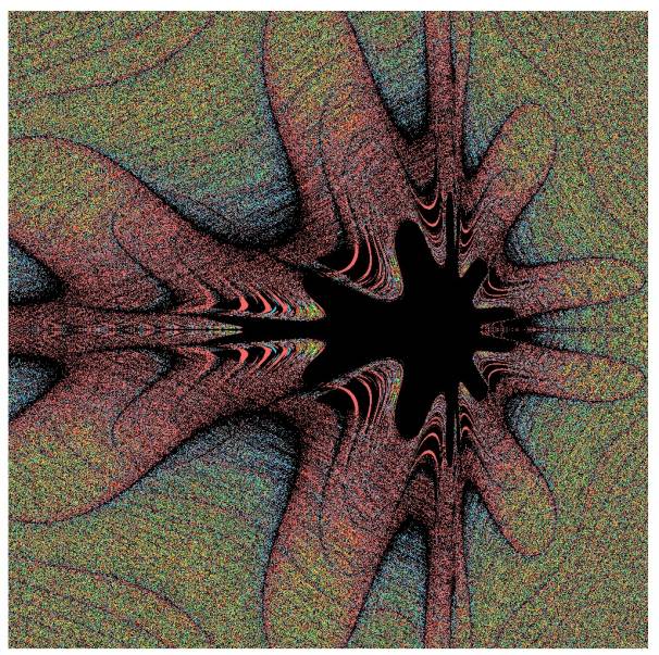
Figure 1. Solution of the 10-parity problem (yellow cells classify more than 531 items correctly; orange cells classify between 519 and 531 items correctly; red cells classify between 515 and 518 items correctly; black cells classify between 511 and 512 items correctly; bleu cells classify between 506 and 509 items correctly, and green cells classify less than 509 items correctly).

 

Once function approximation for functions between an n-dimensional and a one-dimensional space is mastered, the extension to co-domain spaces of dimensionality m>2 is straightforward. This follows from the fact that such a problem can be reformulated as a function approximation problem for a function from an n+m dimensional space to a 1-dimensional space. For this end, the number of training patterns has to be multiplied by m. For every training pattern, the original input-vector is supplemented m times with m additional components. A first time, all additional components are –1 except the first one which is put to +1; the second time, all additional components are –1 except the second one, and so on. If the s-th additional component of such an extended vector is equal to +1, then the target value of this extended vector is equal to the s-th component of the original target vector. In other terms, every additional input dimension singles out a particular output dimension. By activation of this dimension (and non-activation of the other additional dimensions), the output corresponding to this dimension appears at the output unit. Figure 2 shows the demarcation of the S-sets that allow one to solve a 7/6 negation problem and for field definitions related tot he one that led to Figure 1 (see Van Loocke, 1999a for other examples).

 

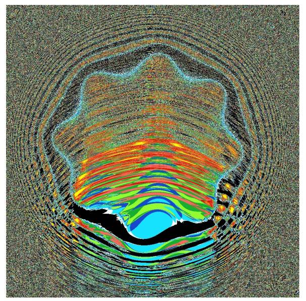
Figure 2. Solution of the 7/6 negation problem

 

 

4. Second illustration of a field definition: IFS-based fields

 

Consider a square part of a plane, and suppose that, for every point (x,y) of this square, a number c(x,y) is defined. The function c(x,y) can be used to define the fields f_i¹,…,f_iⁿ in a cell i if its local properties are exploited. Suppose, for instance, that a problem with a 10-dimensional input space is considered. Then, one can define a set of 10 fields as follows. To start with, one can take f_i¹= c(x_l,y), where x_l is the coordinate of the closest cell to the left of i in the discrete cellular array. Similarly, f_i²= c(x_r,y), where x_r is the x-coordinate of the closest cell to the right of i. With similar notation, f_i³= c(x,y_l); f_i⁴= c(x,y_r); f_i⁵= c(x_l,y_l); f_i⁶= c(x_l,y_r); f_i⁷= c(x_r,y_l), and f_i⁸= c(x_r,y_r). Finally, f_i⁹= c(x_ll,y) and f_i¹⁰ = c(x_rr,y), where x_ll is the x-coordinate of the cell two places to the left, and x_rr is the x-coordinate of the cell two places to the right of i.

 

In order to have fields that are of use when problem solving sets S are constructed, c(x,y) must be sufficiently volatile. For correlations between neighboring values of c(x,y) that are too strong, the statistics of the cells in S deviates too strong from (1)-(3), and no solutions for problems are obtained. On the other hand, c(x,y) must not take a random value in every point when the method is used as a way  to visualize the solutions of complex, high-dimensional classification and function approximation problems. In other terms, a good function c(x,y) has redundancies and correlations that lead to visualizations of adequate quality, but has enough of internal complexity and variation in order to ensure that it can still function as a basis for the construction of adequate sets S.

 

Practice instructs one that IFS-fractals offer a way to obtain such functions. Consider an IFS-attractor for k contraction mappings x’=a_jx+b_jy+c; y’=d_jx+e_jy+g_j  (j=1,…,k). The attractor is a discrete image, and in itself, it is not suited to define a function c(x,y). Nevertheless, it can be used as follows to define a function c(x,y). Consider a series of random integers between 1 and k; suppose the p-th number is denoted h(p). A cell (x,y) is transformed first by the h(1)-th contraction, then by the h(2)-th one, and so on. At every step in this iteration, the distance d between a cell and its next transform is determined and added to a cumulative distance d_c. The iterations run until a point is obtained that is on the attractor of the iterated function system. Then, one puts c(x,y)=cos(e.d_c), with e a system parameter.

 

For many IFS systems, the resulting function contains too much internal correlation to lead to set S that solves problems. However, a simple incremental variation of the algorithm increases the efficiency of the method so that, also for the IFS approach, problem solving sets can be generated. Suppose that the cells of the square are examined from left to right and from top to bottom. Every cell that classifies at least k input vectors correctly is examined. In case of the incremental algorithm, it is included only if the set with inclusion of this cell performs at least as well as the set that had been obtained thus far. Hence, the incremental algorithm defines a subset of the set S that would be obtained in the non-incremental case. This increased selectivity significantly enhances the efficiency of the method. We illustrate this point for the 8-parity problem and for variations of a tree-like IFS (see Peitgen, Jurgens and Saupe, 1992,  p. 295). The non-incremental method does not allow one to define sets that solve the problem. The incremental variation, however, usually does solve the problem after less than quarter of the square has been scanned. Below is a set of 8 Figures giving an impression of the artwork that follows naturally from this problem solving approach. Figures 4, 5 and 7 used sigmoid units to calculate the error function instead of binary units; hence their more smooth and continuous appearance.

 

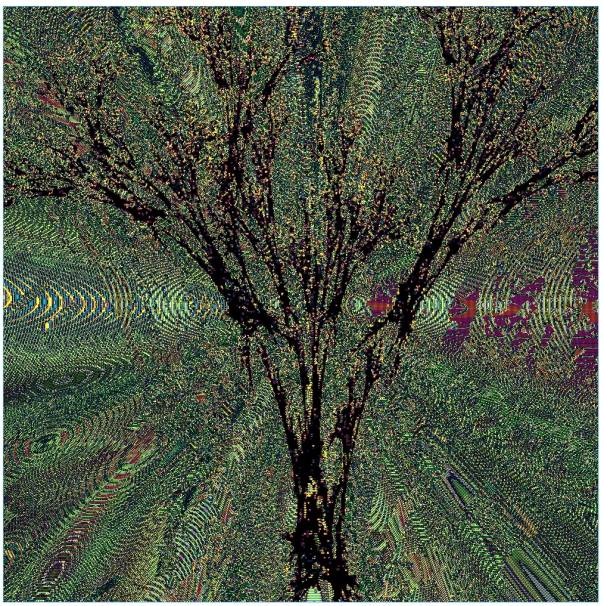
Figure 3. Solution of the 8-parity problem with the IFS method and binary units

 

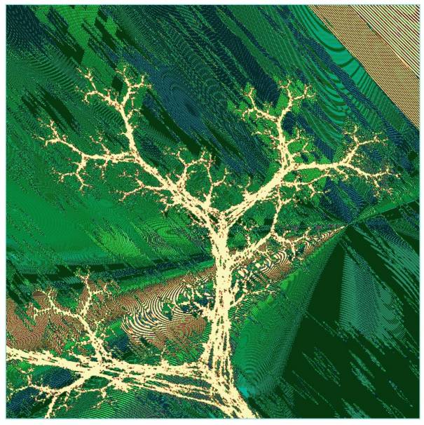
Figure 4. Solution of the 8-parity problem with the IFS method and continuous units

 

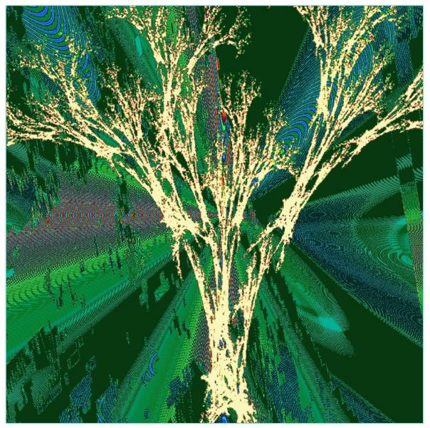
Figure 5. Solution of the 8-parity problem with the IFS method and continuous units

 

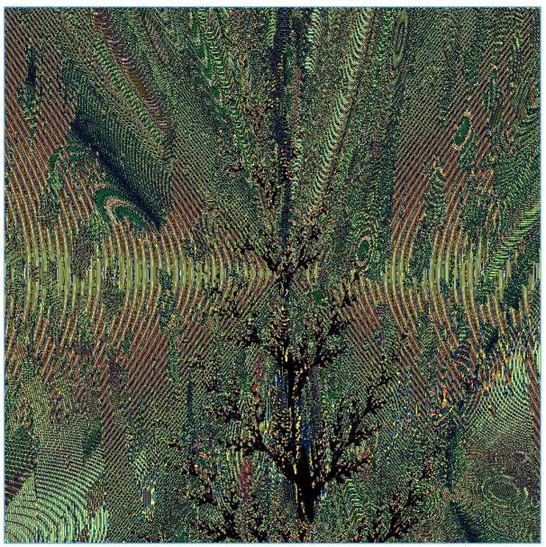
Figure 6. Solution of the 8-parity problem with the IFS method and binary units

 

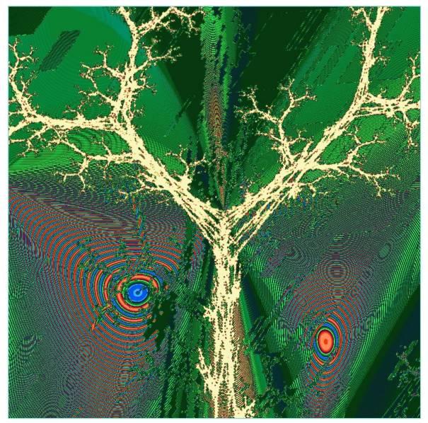
Figure 7. Solution of the 8-parity problem with the IFS method and continuous units

 

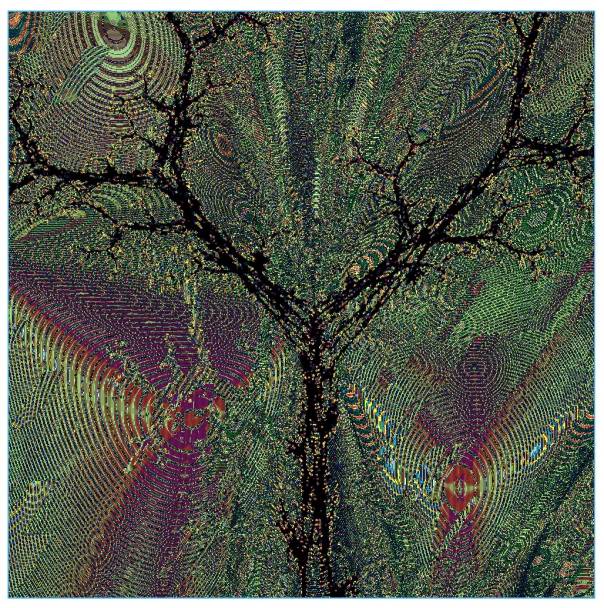
Figure 8. Solution of the 8-parity problem with the IFS method and binary units

 

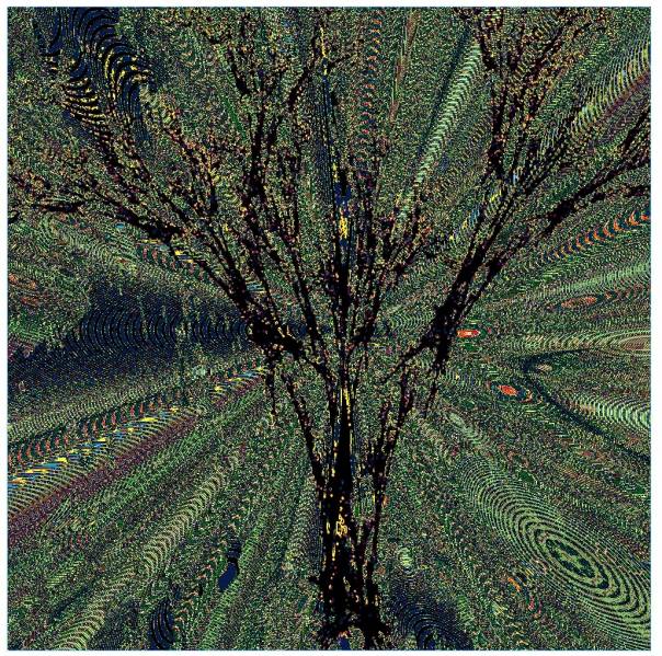
Figure 9. Solution of the 8-parity problem with the IFS method and binary units

 

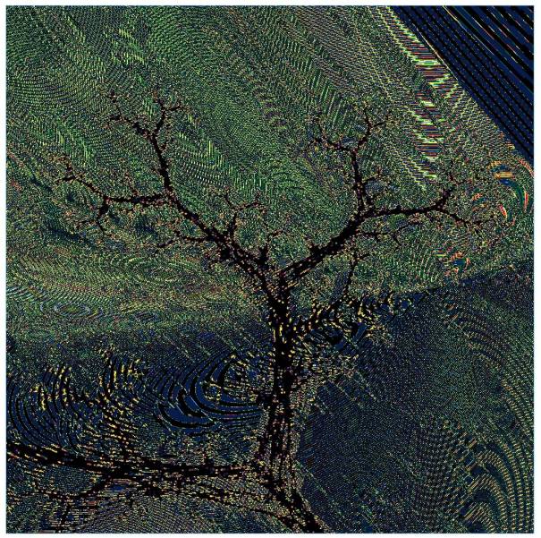
Figure 10. Solution of the 8-parity problem with the IFS method and binary units

 

 

5. Discussion

 

The patterns obtained by the present method can be memorized in a network with a familiar learning rule such as the Hopfield rule, the projection rule, or a Bayesian learning rule (Personnaz, Guyon et al., 1986, Rumelhart and Mc Clelland, 11986, Van Loocke, 1994). Then, one obtains a network for which the memorized patterns correspond to maps between input- and output-patterns. In this sense, such a system memorizes ‘meta-patterns’. This fact can be exploited when one wants to represent patterns with internal structure. First, the internal structure has to be recoded as a function, and subsequently, this function can be represented in the network by the method that has been exposed. (This has been elaborated in Van Loocke (1999a, 1999b) for an incremental algorithm –and for different field definitions. In an incremental algorithm, the cells are considered in serial order, and a cell is included in S only if it reduces the error associated with S. This version of the algorithm also works for continuous-valued dimensions, but the aesthetic quality of the forms is usually lower).

 

As a closing remark, I want to refer to the recent film ‘The matrix’. In this film, people serve as energy for machines. However, they are not aware of this (except for a few heroes), since they are permanently coupled to a giant computer (the ‘matrix’) that generates a virtual reality. The virtual reality is much like our ordinary reality, but for an observer who can observe the people in their capsules, their situation differs profoundly from ours, even though the contents of their consciousness may be similar.

 

We think we are not living in a matrix - we think so. But we see growing forms all around us. We are growing or changing forms ourselves. And we know that growing forms can be used to solve problems (try the present method for a variety of problems and dimensions, and you soon get a gallery of forms with ‘organic’ shape). Suppose we succeed in identifying the problems that are solved by these forms. Then, we could ask if some problem solver, who wanted to solve exactly these problems, had written a simulation in which all these forms are generated. Maybe we participate in the simulation of some godlike being who wanted to solve his problems. In turn, some day we may write complicated simulations in which forms are grown and made to interact in order to solve the very complex problems with which we are confronted. According to the information processing view on consciousness, the entities in this simulation would acquire consciousness, and may consciously perceive their own problems. After some time, the whole story could be iterated one more time, and so on. Of course, this remark is not to be taken serious. Nevertheless, it may be an illustration of the philosophical impact of the sciences of complexity, especially when they are coupled to cognition.

 

 

References

 

Bechtel, W. Abrahamsen, A. (1994), Connectionism and the mind, Oxford: Blackwell

 

Huizinga, J. (1966), Herfsttij der middeleeuwen Amsterdam: Bert Bakker (Translated as: The waning of the Middle Ages (1954), New York, Anchor Books),

 

Leshno, M. Ya Lin, V., Minkus A., Schocken, S. (1993), Multi layer feedforward networks with a nonpolynomial activation function can approximate any function, 6, 861-871

 

Personnaz, L., Guyon, I., Dreyfus, G., (1986), Collective computational properties of neural networks: new learning mechanisms, Physical Review A, 34, 4217- 4228

 

Rumelhart, D, Mc Clelland, J. (eds), Parallel Distributed Processing, 2 Volumes, Cambridge: MIT Press

 

Van Loocke, Ph. (1991), Study of a neural network with a meta-layer, Connection Science, 4, 367-379

 

Van Loocke, Ph. (1994), The dynamics of concepts, Berlin: Springer

 

Van Loocke, Ph. (1999a), Consciousness and the binding problem: a cellular automaton perspective, submitted

 

Van Loocke, Ph. (1999b), Variations of phase fields in cellular automata and aesthetic  solutions for cognitive problems, in Dubois, D. (ed.), Proceedings of the 3-th congress on computing anticipatory systems, New York, American Institute of Physics Press, to appear

 

Yates, F. (1966), The art of memory, London: Peregrin