Human perception and space classification: The Perceptive Network

Mohamed Amine Benoudjit MSc BSc Arch

Christian Derix MSc Dipl Arch

Paul Coates AA Dipl

CECA (Centre for Environment & Computing in Architecture)

School of Architecture & Visual Arts

University of East London, London

Abstract:

This paper presents a computer model for space perception, and space classification that is built around two artificial neural networks (ANN). This model is the first known application in architecture, where a self-organized map (SOM) is used to create a space classification map on the base of human perception criteria. This model is built with the aim to help both the space designers (architects, interior designer and urban designers), and the space users to gain a better understanding of the space in particular, and the environment where they evolve in general. This work is the continuity of an outgoing work started in the CECA by C. Derix around Kohonen network.

Keywords: neural network, self-organised map, perception, space.

1- Introduction:

The main aim of architects is to conceive an adequate environment for human beings. Although this task is usually well fulfilled by architects, we may ask ourselves, how can we be sure that the space as it is conceived through architectural and urban projects, will be accepted by the users and fit their expectancies, if the space designers base their conception only in the way they understand the environment. Conceiving a suitable space means that first we need to define the space and second to find a way to observe it and to understand it as it is perceived by its future users. In other word, to create a tool that substitutes the users by predicting the space based on their perception of it.

Generally, when people think about space, they think about it as the thing enclosed in a building between walls, ceilings and floors:

“… for Scraton, it is self evident that space in a field and in a cathedral are the same thing except insofar as the interior surfaces of the cathedral make it appear that the interior space has distinctive proprieties of it own … space is quite simply what we use in buildings. It is also what we sell. No developer offers to rent walls. Walls make the space, and cost money, but space is the rental commodity” [Bill Hiller, 1996].

This definition could be seen from an architectural point of view as unsatisfactory, because an architectural space is simply more complex, and more sophisticated than the enclosed thing defined by building surfaces. Space has concerned architects and urban designers since the emergence of architecture as an independent field [H. W. Kruft, 1994]. Though, architectural theory considers space as one of its main concerns, it seems that space still hard to define and to situate. This might be due to a difficulty in distilling the essence of the space and to describe it in a universal or a global way. Nevertheless, this does not obstruct some theoreticians to propose definitions for the architectural and urban space, through its historical transformations or through the socio-cultural phenomena that emerge with the evolution of societies on it [B. Lawson, 2001]. Other theoreticians tried to illustrate the space throughout the words, which are used to describe it [R. King, 1996]. This indirect definition of space is due mainly to the following reasons: 1) Human perception is not free from the observer’s emotional content, There fore, the judgement and thus the definition of space might be unsatisfactory, as each individual see it in different way [C. N. Schultz, 1963]. 2) As our environmental experience and space interpretation depend on the purpose of the observation [K. Lynch 1960, Lowenthal and Riel 1970], a global or universal definition of space is hard to achieve.

From above, it appears obvious that: First the definition of space is relative to an individual’s perception from a specific point of and at a specific given time. Second, the only way to fulfil a global, non-personal, objective definition of the space is by understanding the mechanisms underneath the human perception, and the phenomena that influence on it. Once this step is completed, the global definition of the space can be built around the common characteristics of the space, which are shared by all the observers (space users) during the perceptive process.

Following this idea, the computer program we developed is an attempt to illustrate how observers see their space. This is achieved by recreating the abstract representation of the space built by the observer during the perceptive process –during the process of building the space mental images. The program is also an attempt to help both space designers, and spaces users to gain a better understanding of the space, and that by providing them with a space classification and comparison map (Experience 4.d). Our program works in two steps. First, the spaces are analysed in order to extract the global characteristics which define the space and which are common to all observers, such as the physical characteristics of space (size, volume, colour, …). Once this has been done, our program analyses the information extracted by means of a three-dimensional network based on the Kohonen’s self-organizing feature map. Then, it draws an abstract representation of the space under analysis, which will be sent afterward to the classification map (a Kohonen two-dimensional neural network). Finally, the map analyses and classifies those abstract space representations into a two-dimensional self-organized map, which shows the relationship between them.

2- Vision and perception:

Empiric approach of psychology considers vision as the principal motor of perception. In that sense, vision is the active process in which the observer keeps a track of what he is doing, and the process of discovering the external world from a set of visual mental images [D. Marr, 1982]. Those images mapped by the retina, are analysed during the recognition process in order to extract useful information relevant to the objects surrounding the observer or attracting his interest. Then, they are stored in the brain as long-term representations (memories). Observation and scientiﬁc experiments made on normal and brain-damaged people have conﬁrmed that when we think about an object, a mental imagery of its appearance is retrieved based on the long-term memories stored during the object recognition stage [Glyn W. Humphreys, 1999]. These observations and experiences conﬁrmed as well, the inﬂuence of past experiences on the way the world is perceived. The physiological accumulated memories that consist on traces, or representation of the past are added to the new experiences as basic of cultural habits [J. Gibson, 1979]. This means, the perception is function of the individual himself, and that the appearance of the world at any give moment is only a personal expression of that individual.

Kevin Lynch, in his elaboration of a methodology for city design built around the study of the metal images of the visual qualities of the American city, says: “We are not simply observers of this spectacle, but are ourselves a part of it”, and he continues: “Most often our perception of the city is not sustained, but rather partial, fragmentary, mixed with other concerns…”. This environmental mental image is built from the interaction between the observers and their environment, and its main purpose is to cover the need of creating an identity and structure for individuals in their living world. This image can have in different circumstances different meanings. “… An expressway can be a path for the driver, and edge for the pedestrian. Or a central area may be a district when the city is organised on a medium scale, and the node when the entire metropolitan is concerned” [Lynch, 1960]. Thus, the interpretation of the images perceived depends integrally on the purpose of the observer. As a consequence, the only way to achieve a global perception of an environment is by overlapping the individual images of all its users. This public image constitutes a necessity for an individual in order to cooperate with other individuals, and to operate fruitfully within his environment.

Lynch emphasizes that even if each individual has his own mental image of his environment, similarities exist between members from the same group of gender, age, occupation, culture, temperament or occupation. He describes the process by which an environmental image is built and interpreted. The first step for the constitution of the image depends on the distinction and the identification of an object among other things as a separate entity. Then, a set of patterns describing the relation of the object to the observer and to the other objects is added to the mental image already built during the first stage. Finally, personal practical or emotional meanings are added to the object’s mental image [Lynch, 1960].

Likewise Lynch, C. Norberg Schulz points the fact that perception is somehow problematic, because it is not free from emotional contents. He argues that the world is not what appears to us, since we may sometimes judge situation unsatisfactory. “Berkeley argues that qualities of objects depend on the observer’s state”[L. Kaufman, 1974]. Different persons have at the same time different experiences of the same object as the same person can experience differently the same entity at different time depending on his or her attitude at that moment.

“We do all see a house in front of us. We may walk by it, look through the windows, knock the door and enter. Obviously we have all seen the same house, nothing indicates that somebody believed he was standing in front of a tree. But we may also with justification say that we all have different world. When we judge the house in front of us, it often seems as we were looking at a complete different object. The same hold true for the judgment of persons, and not least works of art” [C. Norberg Shultz, 1963].

Judging situations unsatisfactory could often be the result of distortions of the visual space. Sometimes a so-called “geometrical illusions” may occur given the observer a wrong picture concerning his environment or the object of his focus. Traditional theory and experimental psychology divided the geometrical illusions into three categories following the factors that generate them: “A) Certain shapes produce, or tend to produce, abnormal eye movement. B) That some kind of central ‘confusion’ is produced by certain shape, particularly non-parallel lines and corners. C) That figures suggest depth by perspective, and that this ‘suggestion’ in some way distorts visual space” [Richard L. 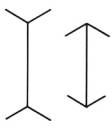Gregory 1963, cited in R. N. Haber, 1968]. Müller-Lyer figures (Figure 1) are a good example to illustrate the destruction phenomena that may influence and modify the retinal image. These figures can be considered, for instance, as the projection of a corner constructed by the intersection of two walls plus a ceiling and a floor. Both left and right figures maybe considered respectively as corresponding to the projection of a room’s corner seen from inside, and a building’s corner seen from outside. Even though, both corners have the same size -the dimension of the vertical lines for the both figures are the same – an illusion is given that the left corner is higher than the right one [Richard L. Gregory 1963, cited in R. N. Haber, 1968].

Figure 1. Müller-Lyer ﬁgures (from Ralph Norman Haber, 1968)

Sedan’s experiences (1932), on blind people that recover their sight after a surgical operation, illustrate that perception is a matter of learning. He reports that after the operation, patients were sometimes capable of differentiating between a cube and a sphere, and sometimes they do not. Those patients start to be seen as normal people capable of distinguishing between shapes and colours after a period of training has occurred. After a period of training of 13 days, a patient was able by counting the corners to discriminate between a triangle and a square. Even though, the training period was short, the patient occasionally shows a capability to recognize those objects from the first glance; the recognition’s mechanism starts to be automatic. An average period of a month is estimated to be sufficient for a full learning [R. N. Haber, 1968].

The new perception’s approach came along with James J.Gibson and his ecological approach. His question about how can we obtain a constant perception of our environment with constantly changing sensations, emphasises the fact that previous philosophical approaches were inappropriate for the definition, and the understanding of the phenomenon of perception [D. Marr, 1982]. His information-based theory considers environmental invariants, from where the senses forward information about valid properties of the environment. “These invariants … correspond to permanent properties of the environment. They constitute, therefore, information about the permanent environment”. Thus, perception becomes “function of the brain, when looped with its perceptual organs, is not to decode signals, nor to interpret messages, nor to accept messages, nor to organize the sensory input or to process the data”. “It is to seek and extract information about the environment from the flowing array of light” [J. Gibson, 1966, 1979].

For Gibson, perceiving is the active process by which knowledge of the world is obtained, and the process by which we keep in touch with our surrounding environment. Although, five sensor systems corresponding to the five perceptual systems (ears, nose, eyes, tongue and skin) work to attain the perception, perception by means of picking up information is achieved mainly through the ocular system (eyes). The amount of information picked by the eyes is function of the observer’s needs. Gibson draws a distinction between sensations and perception. The perception involves meaning and depends on light. It is defined as dimensions of the environment, variables of events, variables of surfaces, places, objects, animals and symbols. On the other hand, sensations depend on the sensitivity and or the use of the sense organs. They are defined as dimensions of qualities and quantities such as extensity and intensity, warmness and coldness. Therefore, the visual perception is not based on having sensations or feelings, but it is based on attention to the information in the light, which is divided into two categories. In one side Gibson defines ambient light as the constant light, which surrounds an individual with an equal intensity. In the other side, he defines optic array or ambient optic array, which is the light that converges from different sources with different intensities. It is viewed as a stimulus of information (Figure 2).

Figure 2. Optical array and its variation following the observer position

(from J. Gibson, 1979)

In the real world, the optic array can be caused by real variation of the light, as it can be caused by the movement of an individual or by an individual whose eyes are moving. Whenever the eyes move to a new stimulation point, a new optical array is created [J. Gibson 1979, E. Reed and R. Jones 1982].

This brief survey of the architectural and psychological literature aims to show the following points: 1) The definition of the perception is a difficult task as each individual perceive his environment in a personalised way. 2) The perception seems to be the result of a long and complex process of learning, where the excitement of certain sensory parts helps in the understanding of the stimulus as an entity. 3) The recognition is the process of perceiving and grabbing specific patterns from their stimulus. Thereby, a global definition of space seems to be difficult to achieve, unless we define it by its influence on the socio-cultural phenomena, or by its physical characteristics. Another alternative is to extract common characteristics to all spaces, shared by the space users during the process of building the space mental images. The following characteristics are some of the common constants shared by all the observers for building the mental images (memories): the dimensions of the space (height, length and width), its colour, enlightenment, the nature of its surfaces and their geometries, and in general all the characteristics that we can measure.

3- The self-organised map (SOM): Algorithm description

In order to make our computer program completely autonomous and self-organized, we have chosen the self-organizing feature map (SOM) as base of development. This unsupervised neural network -conceived by the Finnish neuroscientist Teuvo Kohonen in1982- is defined as a ”nonlinear, ordered, smooth mapping of high-dimensional input data manifolds onto the elements of a regular, low-dimensional array” [T. Kohonen, 2001]. 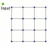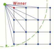In other words, the SOM network, by its specific structure, is a very efficient mathematical algorithm for the extraction of geometrical relationships for a set of objects, and the visualisation of high-dimensional data on a low-dimensional display (two or tri-dimensional display). Based on the human brain, the SOM respects the spirit of competitive learning that exists in the brain between its different neurons, and follows the same path as the biological network concerning the update of the neurons’ weight in the neighbourhood of the winner (Figure 3).


1- Presenting an input point to the network.	2- Localization of the winner neuron, by fining the closet neuron to the input point (use of the Euclidian distance).	3- Update the network following the Mexican hat function. The large amount of update concerns the winner. The neighbourhood update depends on how close it is to the winner.
Figure 3. Competitive learning in Kohonen network

The self-organizing learning of this network consists on, the adaptation of the nodes’ weight after each training cycle in response to the excitation of set of input vectors. The visual representation in this case is known as a topographic map [M. Hassoun, 1995]. The choice of the neighbourhood area is critical. If we start with a small zone, the global ordering of the SOM map will never be reach; instead, the map will stabilize in a mosaic-like shape. The solution proposed by T. Kohonen to avoid this phenomena, is to start with a diameter for the neighbourhood zone bigger that the half of the network. When the map starts to show some order, this radius will be shrink linearly with the time. The ‘time function’ used for the reduction of the radius after each training step does not really matter. Kohonen consider this function a(t) = 0.9(1-t/1000) as a reasonable choice (Figure 4).


a(t)₀	a(t)₁	a(t)₂	a(t)₃
Figure 4. Influence of the winner on the update of its neighbourhood

The initial state of the network is not important for the good functioning of the network’s algorithm (Figure 5a and 5b), the only difference observed between an ordered and a random initial state of the network is a significant decrease in the computational processing in favour of the former state [T. Kohonen, 2001].


Figure 5a.Three frames that shows the organization of a 2D SOM after starting from a random state


Figure 5b. Three frames that shows the organization of a 3D SOM after starting from a random state

The SOM algorithm used in our computer program works as follows. First, the network’s neurons have their weight initialized. Here it is interesting to highlight one of the fundamental characteristics of the SOM, which is that even if the initial weights are same as the inputs, the accuracy of the network is preserved and the final result of the network will be similar to the one with the random weights. The only difference noted between the two ways of setting the weight is that with the similar weight values, the computational time is reduced. Second, the input data fires all the neurons on the network. Then, through a competitive learning, the network designates the neurons, which are the best matches for the fired data inputs. These neurons are denoted as ‘winners’, and the operation by which the winners are found is called the winner-take-all (WTA). The weight updated after each training cycle is assured by a so-called ‘Mexican hat’ function or ‘Neighbourhood’ function (Figure 6); a positive feedback is given to the winners and their neighbours as defined by the neighbourhood function, and a negative feedback is given to the rest of the neurons. In other word, the neurons within the area defined by the neighbourhood function are slightly excited, and thus have their weight updated in function of how far or close are they to the winners; the closer to the winners they are the closest their updates are to those of the winners. This process is repeated a couple of times until the full learning of the network is reached. Kohonen suggests for a good statistical accuracy that the number of training steps should be at least 500 times the number of nodes in the network [T. Kohonen, 2001].

Figure 6. Neighbourhood function or Mexican Hat function

4- Experiments

All the above experiments are based on Visual Basic for Application scripts running under AutoCAD 2000 or higher versions.

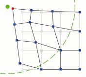
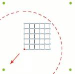
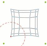
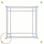
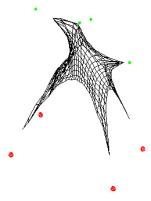
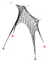
4.a The Magic Carpet

The magic carpet was the first experimentation made with Kohonen network for space representation. Inspired from Kohonen’s ‘Magic TV’ experiment (for more information refers to Kohonen’s book), the idea behind it was to understand the mechanisms underneath his algorithm, and to see the possibilities of using it for the space perception. The main difference between a traditional SOM and the ‘Magic Carpet’ algorithm is while a traditional SOM is only used as an analytic tool, which represents the network nodes, the ‘Magic Carpet’ go beyond that by using the map also as a display tool. There fore, for the training of the network, we considered the training points as a set of three vectors, which defines their position into the Euclidian space (X, Y and Z coordinates). In this experiment, the training points (data inputs) are divided into two groups. The first group is composed by the red training points, which are always situated underneath the map at its extremities. The second group of data inputs is represented by the green balls, drawn by the algorithm at random position above the network. Both the size of the network, and the number of training points above the network (the green balls) are chosen by the user at the runtime.

Once the training points are presented to the network, the map or network starts to adjust itself after each training cycle, and this by updating the coordinates of its nodes (neurons), until it settles down with a geometrical configuration close to the shape represented by those training points.


T = t₀	T = t₁	T = t₂	T = t₃
Figure 7. The Magic Carpet: implementation of a third dimension to a 2D map

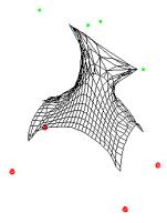
The positive point about the ‘Magic Carpet’ algorithm is the ease, and the rapidity by which the surfaces are generated from an initial set of points. Though further development of the program may be needed, this tool could be seen as a good alternative for building organic shape in comparison with other tri-dimensional software, because here the user has only to input the points that define the organic shape that he is after rather than to model it all by himself.

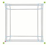
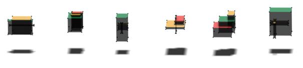
4.b The Five Dimensional Map

The idea here was to experiment how the map network will behave, in the case where the input points are defined by more than tri-dimensional vector. In this experiment, in order to provide an easy reading of the map, and in order to judge the global behaviour of map, we used as network’s neurons balls instead of the mesh vertices such was the case for ‘The Magic Carpet’ experiment (Figure 8). The five dimensions of the network are defined as follows:

- The X, Y and Z coordinates for each neurons and each training point represent the three first dimensions.

- The forth dimension represents the initial size of the ball for both neurons and input points.

- The fifth dimension represents the initial colour for both network neurons and input points.

The network nodes are initialized with different sizes and colours. The set of input points presented to the network consists on height balls with different size, four below the network (map) and four underneath the network (Figure 8.T = t₀). The colour for these balls was the same. The purpose of this choice was to provide us with some input vectors that can be controlled. This enables us to have a control over the network and helps us to evaluate if the algorithm is working properly or not. Same as in the previous experiment, the training points underneath the map are drawn automatically by the program, and those above it and the size of the map is controlled by the user at runtime.

Once the training period is over (Figure 8.T = t₃), we observe the following:

- The organisation of the neurons on the space follows the shape designed by the training points.

- The network nodes present a certain order concerning their colours and their sizes. More the nodes are close in distance to the training points, more their sizes and colours become similar to those of the training points. This phenomenon can be observed in (Figure 8) where network’s nodes of similar sizes and colours are gathered around the training points.

This is explained by the way the network is trained and the way we get feedback from it. In this experiment, once the winners are selected by the network’s algorithm, their Euclidian position in the space, their colour and thus their size are updated following the rules of the WTA and the ‘Neighbourhood’ function.


T = t₀	T = t₁

T = t₂	T = t₃
Figure 8. The Five Dimensional Map

Not all our expectations have been reached in this experimentation. When we were elaborating the algorithm, we expected to end up with a map that contains a large variety of colours, and that the transition from one colour to others will be assured by intermediate nuances. Although, numerically speaking, the algorithm works fine, and certain logic exists in the way we pass from on colour to the one beside it, this order is not present on the visual display of the map; we can easily observe a discontinuity in the transition between the different colours. This is due to the limitation on the number of the colours to 256 colours in AutoCAD, and to the way they are built on it.

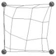
4.c Calibrated Map

One of the main characteristic of the self-organised map (SOM) is its capacity to classify objects or any other kind of data within a map. This organisation of the map does not need an additional training of the network, it just needs to pass the network nodes through a calibration process, which consists on labelling the neurons with their analogue training inputs. Thus, a self-organized map is built.

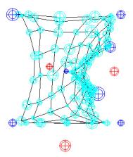
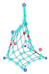
In order to illustrate the calibration process, we used in this experiment a four-dimensional network where the neurons are represented by the cyan balls, and the training input by seven blue balls (Figure 9). The four dimensions of the network are as follows:

- The three first dimensions are represented by the X, Y and Z coordinates of both input points and network nodes.

- The fourth dimension consists on the size of the neurons and the input points.

The ‘Figure 9. T = t₀’ represents the end of the training process. Once the training was over we presented to the network three more samples (the calibration points), which are represented in the ‘Figure 9. T = t₁’ by the red coloured balls. The map compares its nodes with the calibration points, and changes the colour of the nodes that match the calibration points into red (Figure 9. T = t₂).

T = t₀

T = t₁

T = t₂

Figure 9. Self Organized Map Calibration

4.d The Perceptive Network

The following experiment is the collection of the previous ones with as an add-on the introduction of human being perception criteria. The algorithm in this experimentation flows as following:

1- A set of offspring is generated by a genetic algorithm where each one of them is composed of three boxes. Here each offspring could be thought as a distinct spatial configuration (Figure 10).

Figure 10. Generation of a set of spaces by the use of a genetic algorithm

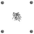
1-For each space, the coordinates of its vertices are collected in order to build the training inputs that will be presented to the network in the next step. The vertices are marked by small coloured balls as shown in ‘Figure 10’.

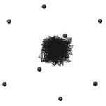
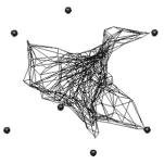
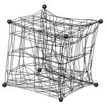
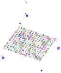
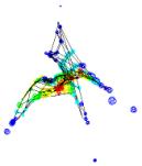
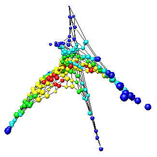
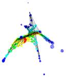
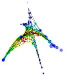
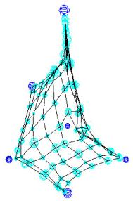
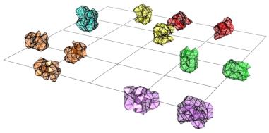
2-The program affects to each space a tri-dimensional network (3D SOM). The initial state of 3D SOMs is the same for each space: a cubic network. After a short training period, each 3D SOM starts to take a geometrical configuration different from the others (Figure 11).

3-The 3D SOMs created after the training cycle, are the abstract representation of the spaces created in the first step. Those abstract representations are based on the human beings perception.


Figure 11. Generation of the tri-dimensional self-organized maps (3D SOMs)

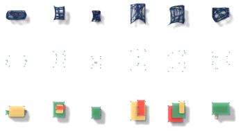
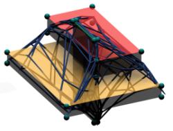
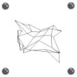
4-As the cubic networks are composed only by nodes and lines –nodes for the representation of the neurons and the line for the representation of the interconnection between the neurons- a clear reading of the abstract forms generated by the networks is difficult. In order to make the reading easier, we used a marching cube algorithm that creates shells (isomorphic geometries) around the 3D SOM based on its neurons (Figure 12).

A similar technique has been used by C. Derix with his early experiments with Kohonen’s neural network (P. C. Coates and al, 2001).

Figure 12. Generation the abstract representation of the spaces

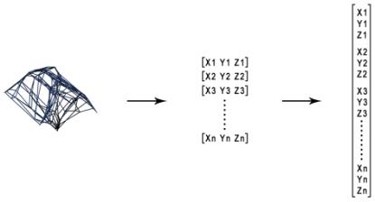
5-Once, all the abstract representations have been generated by the marching cube algorithm, the coordinates of all the 3D SOMs’ neurons are collected, and used to build the matrices (Figure 13) for the training and the calibration of the space self-organized map (2D SOM).

Figure 13. Building the matrices for the training of the 2D SOM

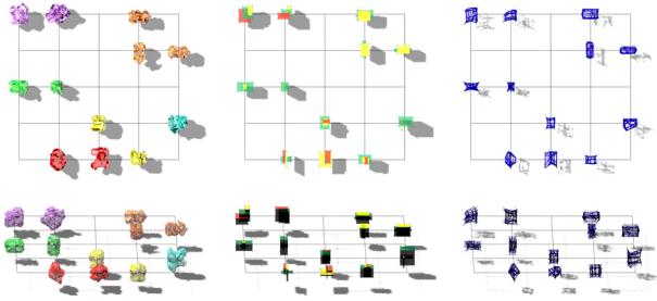
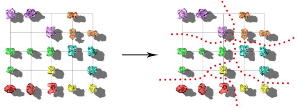
6-In this step, the 2D SOM is trained and a 2D map is generated classifying in the meantime all the 3D SOMs generated in step 2 (Figure 14). This map has the characteristic to situate similar spaces in the same area of the map, and different spaces in different areas of the map.

In this map we start to observe the emergence of groups according to their similarities. This kind of organisation is similar to the way the human brain stores information.

Figure 14. Training and calibration of the 2D SOM

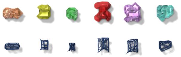
7-To make the comparison between the spaces easier for the user of the algorithm, two additional maps are created; one based on the initial forms generated by the genetic algorithms, and a second composed by the abstract representation of the spaces that are created by the artificial neural network (Figure 15).

Figure 15. Building the classification map based on the spaces and the 3D SOMs

8-Using the genetic algorithm again, a new set of spaces is generated, and presented to the 2D SOM in order to classify them (Figure 16) through the calibration process.

Figure 16. The space classification map

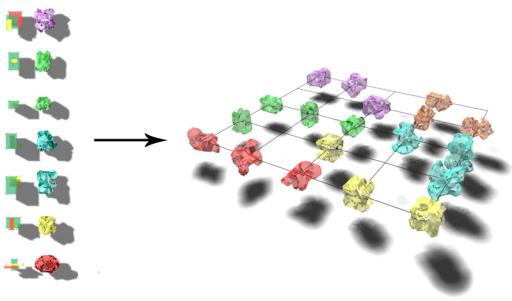
The organisation and the subdivision of the space self-classification map become more evident in the newly created map in comparison to the map generated in the ‘step 6’ of this experiment.

Figure 17. Organization of the spaces on the map as groups

Observations and ideas for future work

The algorithms described in this paper are new alternatives for the use of artificial neural network in architecture, in order to understand, project and design spatial configurations. The use of Kohonen’s network among other computing techniques appears to be a very good choice. Though the number of computations is very high, in particular if we use more than three boxes to describe the different spatial compositions, the program computes rapidly and smoothly, regardless of the computer power used for the computational process.

Although the program is still under development, the results we get for the space classiﬁcation are very promising. The next step will be to improve this program by implementing more criteria to the neural network algorithm:

a- Use of the Dot Product and the Learning Vector Quantization (LVQ) instead of the Euclidian Distance in order to define the winners. Once this is achieved the result will be compared to those obtained with the Euclidian Distance in term of accuracy and computational speed.

b- At the present time, the only output we get from the program is a visual classiﬁcation of the space under study. It will be interesting to improve the program in such a way that we obtain more feedback concerning the qualities of the space.

c- The other interesting step for future work is to use more accurate criteria for the definition of the space such as: the dimension of the space, its volume, the characteristics of its objects and components, its colour, enlightenment, the nature of its surfaces and their geometries.

Another interesting point to develop is to build other computer programs based on other mathematical models, such as the support vector machine, and compare their results with those obtained with the SOM.

References

Geoffrey Broadbent, Richard Bunt and Tomas Llorens (1980). Meaning and Behaviour in the Built Environment. John Wiley and Sons, UK.

Paul Coates, Christian Derix, Tom Appels and Corinna Simon (2001). Three Projects: Dust, Plates & Blobs. Centre for Environment and Computing in Architecture CECA, Generative Art 2001 Conference.

Christian Derix (2004). Building a Synthetic Cognizer. Poster for the MIT Design Computational Cognition 2004 Conference, USA.

Education in Computer Aided Architectural Design in Europe eCAADe17 (1999). Architectural Computing From Turing to 2000. The University of Liverpool, Liverpool, UK.

James J. Gibson (1966). The Senses Considered as Perceptual Systems. Houghton Mifflin, Boston, USA.

James J. Gibson (1979). The Ecological Approach to the Visual Perception. Houghton Mifﬂin, Boston, USA.

Kevin Gurney (1997). An Introduction to Neural Networks. UCL Press, London, UK.

Ralph Norman Haber (1968). Contemporary Theory and Research in Visual Perception. Holt, Rinehart and Winston, USA.

Hermann Haken (1978). Synergetics: An Introduction. Springer, Berlin.

Mohamed H. Hassoun (1995). Fundamentals of Artiﬁcial Neural Networks. A Bradford Book, MIT Press, Cambridge, London, Great Britain.

Bill Hillier (1996). Space is the Machine: A Conﬁgurational Theory of Architecture. Cambridge University Press, London, UK.

J. H. Holland (1992). Adaptation in Natural and Artiﬁcial Systems: An Introductory Analysis with Applications to Biology. Control and Artiﬁcial Intelligence, MIT Press, Cambridge , UK.

Glyn W. Humphreys (1999). Case Studies in the Neuropsychology of Vision. Psychology Press Ltd, UK.

George Johnson (1986). Machine of the Mind: Inside the New Science of Artiﬁcial Intelligence. A Tempus Book from Microsoft Press, USA.

Lloyd Kaufman (1974). Sight and Mind. Oxford University Press, London.

Teuvo Kohonen (2001). Self-Organizing Maps. 3rd Edition, Springer, Germany.

Hanno-Walter Kruft (1994). A History of Architectural Theory From Vitruvius to the Present. Zwemmer, London.

Bryan Lawson (2001). The Language of Space. Architectural Press, Oxford, Great Britain.

Kevin Lynch (1960). The Image of the City. Twenty height printing (2002), Joint Center for the Urban Studies, USA.

David Marr (1982). Vision. W.H. Freeman, USA.

James V. McConnell (1974). Understanding Human Behavior. Holt, Rinehart and Winston, USA.

Marvin Minsky and Seymour Papert (1972). Artiﬁcial Intelligence. The MIT Press Cambridge, Massachusetts.

Michael J. Morgan (1977). Molyneux’s Question: Vision, Touch and the Philosophy of Perception. Cambridge University Press, London.

Rolf Pfeifer and Christian Scheier (2001). Understanding Intelligence. The MIT Press, Cambridge, Massachusetts, USA.

Vernon Pratt (1987). Thinking Machines: The Evolution of Artiﬁcial Intelligence. Basil Blackwell Ltd, Oxford, UK.

Edward Reed and Rebecca Jones (1982). Reasons For Realism: Selected Essays of James J. Gibson. Lawrence Erlbaum Associates LEA Publishers, London.

C. Norberg Shultz (1963). Intensions in Architecture. Aristide, Staderini, Rome, Italy.

John A.K. Suykens, Joos P. L. Vandewalle and Bart L. R. DeMoor (1996). Artiﬁcial Neural Networks for Modelling and Control of Non-Linear System. Kluwer Acadimic Publishers, Netherlands.

Ali .M.S. Zalzala and A.S. Morris (1996). Neural Networks for Robotic Control: Theory and Applications. Hartnolls Limited, Great Britain.

Dave Anderson and George McNeil (1992). Artiﬁcial Neural Networks Technology. Data & Analysis Centre for Software, Room Laboratory, DoD DACS [online].

Available from: http://www.dacs.dtic.mil/techs/neural/ [13-06-2004].

Lesley Smith (2003). An Introduction to Neural Network. Centre for Cognitive and Computational Neuroscience [online].

Available from: http://www.cs.stir.ac.uk/~lss/NNIntro/InvSlides.html [13-08-2004].

Chris Stergiou (1996). What Is a Neural Network? [online].

Available from: http://www.doc.ic.ac.uk/~nd/surprise_96/journal/vol1/cs11/article1.html [05-07-2004].