Non-linear projection of IFS attractors: symmetry breaking and symmetry restoration
Philip Van Loocke
Department
of Philosophy
University of Ghent
Blandijnberg 2, Ghent 9000,
Belgium
philip.vanloocke@Ugent.be
Yannick Joye
Department
of Philosophy
University of Ghent
Blandijnberg 2, Ghent 9000,
Belgium
yannick.joye@Ugent.be
Abstract. A method is proposed in which iterated
function systems are combined with non-linear tree projections. A form is
initialized by a linear tree which projects to the attractor of an iterated
function system. Curvature fields are associated with the line segments of the
tree, by which a non-linear, three-dimensional form is obtained. Then, a method
is proposed that breaks the symmetry of the resulting form at different levels.
After symmetry-breaking, an operation of symmetry restoration can be applied in
order to obtain forms in which branches converge to a limited set of points.
1. Linear projection of an
attractor of an iterated function system
Consider the Sierpinski triangle in Figure 1. It is
obtained as the attractor of the iterated function system defined by the
transformations f 1, f 2
and f 3 which transform the plane into itself, and with f
x1(x, y) = 0.5 x; f y1(x,
y) = 0.5 y; f x2(x, y) = 0.5 x + 0.5; f y2(x,
y) = 0.5 y; f x3(x, y) = 0.5 x + 0.25; f y3(x,
y) = 0.5 y + 0.5. Suppose that an initial point R is randomly chosen in the
unit square. If this point is subject to a large number of transformations from
the set {f 1, f 2, f 3}, and if these are
applied in random order, then the entire figure appears (if the initial point
is not on the attractor, the first few tens of iterations are to be left out of
the figure). This is the usual way to generate attractors of iterated function
systems. Figure 1 was generated in a different way. The initial point R had
coordinates (0.5, 0.5). Then, this point was subject to all combinations of
eight transformations fk1◦fk2◦…◦f
k8 (with k1,…,k8 = 1,…,3), so that 38 =
6561 points were generated. Suppose that the point obtained after application
of a particular combination fk1◦fk2◦…◦f
k8 on R is denoted Pk1,k2,...,k8. The first index of this
point corresponds to the transformation which is applied last. Its predictive
value with respect to the location of the point is largest: it specifies that
the point is on the k1-th transform of the attractor. The second
index refines this place: the point is on k1-th transform of the k2-th
transform of the attractor, and so on. Therefore, points differing in the last
index k8 only are close to each other; points are usually further
removed if more early indexes are different.
A linear, ternary tree of which the endpoints coincide
with the points on the Sierpinski triangle is generated in two stages. First,
the tree is constructed in the plane of the triangle. Subsequently, the
starting point S of the tree is moved out of this plane, while the endpoints of
the tree are remaining at their place. Intermediate branching points are drawn
toward S as a function of the branching level. In the second stage, a
three-dimensional linear tree is generated by connecting all lower level
branching points with the three corresponding higher level points (Figure 3).
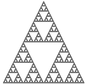
Figure 1. Points
on the Sierpinski triangle obtained by combination of eight transforms
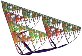
Figure 2. Three
dimensional linear tree-projection of the Sierpinski triangle
2. Definition of fractals
fields over the attractor of an iterated function system
Consider the point Pk1,k2,...,k8 on the
Sierpinski triangle. A field f k1,k2,...,k8 is defined as
a function of the value of the indexes k1,…,k8. The
general form of this function reads:
f k1,k2,...,k8 = S{s=1,...,8} bs,ks (1)
This expression means that, for each of the eight
transformations involved in the definition of
Pk1,k2,...,k8, fk1,k2,...,k8 is increased by a
quantity bs,ks (s=1,...,8; ks=1,...,3). The quantities bs,ks
depend on the level s for which ks specifies the transformation, and
on the value of ks itself. For the present choice of eight levels,
and of an iterated function system defined by three transformations, this means
that the field expression (1) includes 3.8=24 parameters. Variation of these
parameters leads to different fields, and hence in the next section to
different non-linear forms.
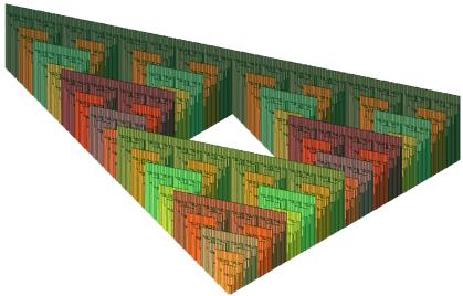
Figure 3. Field defined by bs,ks=1 if ks=1
or ks=2, and bs,ks=3 if ks =3
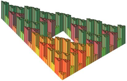
Figure 4. Field defined by bs,ks = Rnd.
(9 – s)6, and with symmetrization
3. Generation of non-linear
forms by field-induced curvature
In order to insert curvature in a linear tree, it has
to be analyzed into spatial variables. Because of the fact that we want fields
to directly induce curvature, a tree will be described in terms of angular
variables which are associated with line segments. Consider the s-th level branch with endpoint Pk1,k2,...,ks (s=1,…,8). Suppose that this branch is
divided into N segments of equal length. The unit vector along the n-th line
segment is denoted enk1,k2,...,ks (n=1,...,N). This vector is specified by two
angles (qnk1,k2,...,ks, jnk1,k2,...,ks),
where q nk1,k2,...,ks is the angle between the x-axis and the
projection of enk1,k2,...,ks on the horizontal plane, and
j nk1,k2,...,ks is the angle between the z-axis and enk1,k2,...,ks. For all segments along the branch
(except for the first segment), the differences in angles can be determined: dqnk1,k2,...,ks = q nk1,k2,...,ks – q n-1k1,k2,...,ks ; dj nk1,k2,...,ks = j nk1,k2,...,ks – j
n-1k1,k2,...,ks (n=2,...,N) (see [1]).
By coupling these differences to fields, the trees are
made non-linear. Two fields in agreement with the previous section are taken.
These are coupled with the horizontal and the vertical differences in angles,
respectively.
dq nk1,k2,...,ks = dq nk1,k2,...,ks
+ a f
hk1,k2,...,ks ;
dj nk1,k2,...,ks = dj nk1,k2,...,ks + b f vk1,k2,...,ks
(a and b are coupling constants)
The quantities fhk1,k2,...,ks are
called horizontal fields; they give horizontal curvature to the linear
branches. Similarly, the quantities fvk1,k2,...,ks curve
branches by modification of the angles of line segments with the z-axis.
The procedure in which trees are curved by fields can
be iterated. After an object is obtained by coupling of fields to angular
differences, a linear tree can be constructed so that its final level endpoints
coincide with the final level endpoints of the object. Then, this linear tree
can be curved in accordance with field definitions, and so on. After a few
iterations, this process usually leads to forms of high complexity. Figure 5
was generated for three iterations. Figure 6 illustrates a run of the program
in which vertical fields included a harmonic factor of horizontal angles. In Figure
7, all fields included a harmonic factor of vertical angles
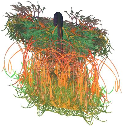
Figure 5. Form obtained after three iterations
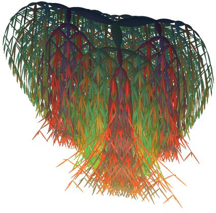
Figure 6. Run of program for vertical fields with
harmonic factor of horizontal angles
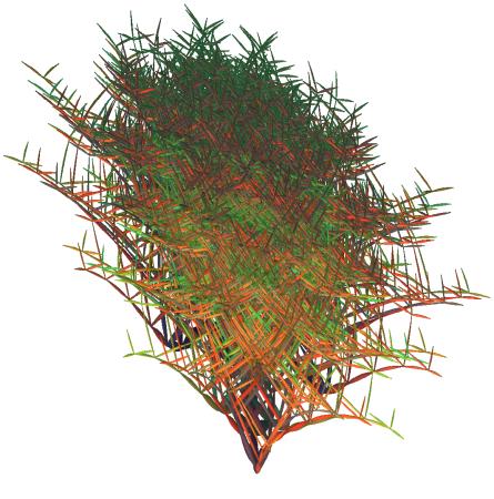
Figure 7. Run for fields with harmonic factor of
vertical angles
4. Symmetry restoration
Suppose that, in some or other context, one aims at a
form that has less divergence of endpoints. This can be obtained by an
operation in which endpoints are drawn together in sets of 3k points. Subsequently, branching
nodes at lower levels are moved in proportion with the average movement of
higher level nodes. Consider the form in Figure 8. For k=1, the first stage in
the convergence process is obtained; it is shown in Figure 9. At final stage,
all endpoints point to the same point, as is illustrated in Figure 10.
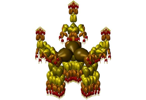
Figure 8. Initial form before symmetry restoration
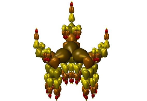
Figure 9. First stage of convergence process
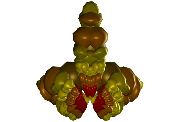
Figure 10. Final stage of convergence process
References
[1] Van Loocke, Ph. (2004), Data visualization with fractal growth, Fractals, 12(1), 123-136