Generating Images
Using Solar System Kinematics Parameters
B. Soban, BSc
Freelance Generative Artist.
e-mail:
bogdan@soban-art.com, www.soban-art.com
Abstract
Random numbers play an important role inside program
algorithms which create artworks using an autonomous generative process.
Practically two types of random number generators are used: computational and
physical. In this paper the use of the solar system as a source for a physical
random generator is described and used inside the experimental generative
program. The planets revolving around the sun produce an immense number of
variables which are used as the dynamic parameters inside mathematical
equations resulting in random numbers. To make the system more complex the
dynamical drawing point based on a pulsing spiral curve is applied. The same
source of random numbers is used to create the set of coloring palettes by
corresponding algorithms. The program is partially controlled from the outside
with a possibility to change any parameter during the execution. Resulting
images are pure abstract artworks, color harmonized and with perceived central
orientation. Observing generated images and knowing the fact that only a little
part of solar system variables was used for the described experiment, the
approach could represent a great challenge in the future to develop more
complex programs producing a new kind of art inside a generative concept.
1. Introduction
The outside
influence on a generative art process is one of the main characteristics which
distinguishes them as absolutely autonomous or partially interactive. An
autonomous concept doesn’t permit any kind of outside intervention and the
result depends exclusively on random number generators and complex algorithms.
To develop such a program without the use of a random number generator is not
an easy task and could be an interesting challenge. To find another system to
produce useful random values without a random number generator was the basic
idea of the project presented in this paper. Taking into consideration that
machinery engineering is my basic education the kinematics systems have
appeared useful. The real possibility could be the simulation of an existing
kinematics system and to use its continuously changing variables as input into
a generative process. In the beginning I have analyzed a very simple system
which transformed linear motion into rotation. A very typical and to everybody
known example is a steam engine but it produces a very limited number of
variables to be a good source for a random number generator. So I decided to
use our Solar system which is more complex in producing different variables.
Our solar
system with all his planets and other bodies revolving around the sun is a
problem that has perplexed mathematicians and astronomers since antiquity,
especially in connection with the theory of chaos. According to the Greek
mathematician Pythagoras, the Earth and the planets revolved around the Sun,
producing musical notes as they moved, from which we derived the expression
“the harmony of the spheres”. Studying the chaos theory based on anomalies of
the solar system has developed the idea to draw complex pictures that arise
from a chaotic system – in this case from the Solar system [1].
The motion of
planets around the Sun produces a lot of parameters as positions, angles,
distances, velocities etc, which could be used to define all necessary elements
to generate an unpredictable and never repeatable image. In order to generate
interesting images it was enough to use only distances between planets or the
sum of distances from a selected planet to all others or the sum of all
possible distances between all of them. To realize the experiment in an easier
way it was necessary to introduce some simplifications: circles as the planet
orbit, higher but proportional angle speed and random starting position. In
order to realize this experiment I have developed a generative program where a
random number generator is used only to define the planet’s starting position.
All other elements used to draw an image are calculated out of variables
produced by the solar system simulation in the background.
2. Solar systems overview
The solar system consists of the Sun, the eight official planets, at
least three dwarf planets, more than 130 satellites of the planets, a large
number of small bodies (the comets and asteroids), and the interplanetary
medium. There are probably also many more planetary satellites that have not
jet been discovered. The inner solar system contains the Sun, Mercury, Venus,
Earth and Mars. The main asteroid belt lies between the orbits of Mars and
Jupiter. The planets of the outer solar system are Jupiter, Saturn, Uranus, and
Neptune. Pluto as the ninth planet is now classified as a dwarf planet [2].
Relative orbits of the sun and the nine planets are shown in Figure 01.
figure
01
The planets, most of the satellites of the planets and the asteroids
revolve around the Sun in the same direction, in nearly circular orbits. When
looking down from above the Sun’s north pole, the planets orbit in a
counter-clockwise direction. The planets orbit the Sun in or near the same
plane, called ecliptic. The ecliptic is inclined only 7 degrees from the plane
of the Sun’s equator. Pluto is a special case in that it’s orbit is the
most highly inclined (18 degrees) and the most highly elliptical of all the
planets. Because of this, for part of its orbit, Pluto is closer to the Sun
than is Neptune. The axis of rotation for most of the planets is nearly
perpendicular to the ecliptic.
Statistical information for the planets generally consists of the mass,
equatorial radius, mean density, mean distance from the sun, rotational period,
orbital period, mean orbital velocity, orbital eccentricity, tilt of axis,
orbital inclination and others [3]. For the purpose of my research only some of
them could be useful. The selection property was that the data is not a
constant or that the relation between the same data of different planets is not
a constant. For example, the sum of the mass of all the planets is a constant,
but the sum of the distances between all the planets is a permanently changing
variable. So I have selected the distances between planets as the basic
platform for all my calculation needs. For this purpose there are necessary two
set of data: the mean distance from the Sun in AU (astronomical unit – the
distance between the Sun and the Earth) and the orbital period in years. Table
01 presents real data used in the simulation program.
|
|
Mercury |
Venus |
Earth |
Mars |
Jupiter |
Saturn |
Uranus |
Neptune |
Pluto |
|
distance |
0.39 |
0.72 |
1.0 |
1.5 |
5.2 |
9.5 |
19.2 |
30.1 |
39.5 |
|
period |
0.24 |
0.62 |
1.00 |
1.88 |
11.87 |
29.46 |
84.01 |
164.79 |
248.54 |
Table
01
3. Simplifications
In order to realize the experiment I developed a special generative
program in Visual Basic. The program consists of two parts: a dynamical
simulation of the solar system in the background and a generative part of the
program which uses the simulation as a random number generator to produce
variables needed to generate images. To make the simulation easier but good
enough to reach the defined scope I had to use some simplifications: all
planets orbit in the same plane and they revolve around the sun in circular
orbits. I have eliminated all moons, asteroids and comets although those bodies
and their motions could be very useful to make a random number generator
better. I have preserved the real distances between the Sun and the planets and
relative orbital period adapted in a way, that Pluto makes the whole round in
some minutes when the program is running. The other planets make their own
rounds regarding their orbital period. For example: during one Pluto round the
Earth makes 248 rounds. Figure 02: Planet’s orbits as circles in a proportional
scale.
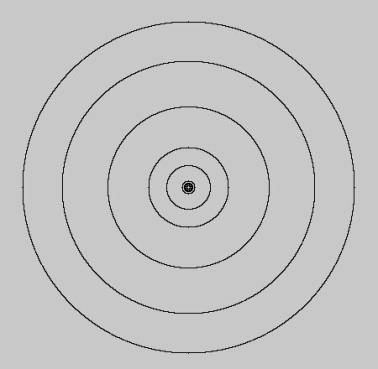
Figure
02
During the first experiments with the program another
problem appeared. The real position of the planets according to the real date
and time as the starting position for the simulation didn’t give good results.
Using the random number terminology, the phenomena could be explained as the
same seed in every program cycle. It means that program generated every time
the same set of images. One minute of time is too short to perceive any
difference in the relative position of the planets. It is natural that the
absolute move in km is enormous but in relative correlation infinitesimal.
Introducing one-year period for inner planets gives a good result, while for
the outer planets not satisfying. Figure 03 presents four positions of planets:
now, one-year before, ten years before and hundred years before
(28.10.2006/2005/1996/1906) [4].
Figure 03
A short analysis of planets’ position during the time
definitely eliminated the idea of applying the real time planet position in the
simulation. So I introduced another simplification: every program start defines
an absolutely random planet position using RND function. This is the only case
where the RND function is used inside the program. All other random values
needed are calculated from the solar system simulation.
4. Solar system as the
source for a random number generator
Random numbers have essential meaning for generative
art programming. All “decisions” in the program algorithm are dependent on
different values which are usually random. A random number is a number generated
by a process whose outcome is unpredictable and which cannot be subsequently
reliably reproduced. This definition works fine provided that one has some kind
of a black box – such a black box is usually called a random number generator –
that fulfills this task [5]. A random number generator is a computational or
physical device that produces sequences of numbers complying with the
definitions proposed above. There exist two main classes of generators:
software and physical generators. From a general point of view, software
generators produce so-called pseudo random numbers. Although they may be useful
in some applications, they should not be used in most applications where
randomness is required. Most pseudo random generators generate a sequence of integers
by the following recurrence:
X(0) = given,
X(n+1) = P1 * X(n) + P2
mod N
Parameters P1,
P2 and N determine the characteristics of the random number generator and the
choice of X(0) – the seed – determines the particular sequence of the random
numbers that is generated. If the generator is run with the same values of the
parameters and the same seed it will generate a sequence that is identical to
the previous one. The approach and formula described above has an essential
weakness: once the generator generates a number which was generated before the
whole sequence then repeats itself [6].
In applications where pseudo-random numbers are not
appropriate one must resort to using a physical random number generator. When
using such a generator it is essential to consider the physical process used as
a randomness source. This source can be either based on a process described by
classical physics or by quantum physics. A physical random number generator is
based today on an essentially random atomic or subatomic physical phenomenon.
Examples of such phenomena include radioactive decay and thermal noise [7].
Frequently used term is hardware random number generator. This is a piece of
electronics that plugs into a computer and produces genuine random numbers. The
usual method is to amplify the noise generated by a resistor o a semi-conductor
diode and feed this to a comparator. The output is a series of bits which are
statistically independent. These can be assembled into bytes, integers or
floating point numbers and then into random numbers [8]. A registered noise from the street
transformed into digital data could be a very useful random number source.
In my case the solar system with its kinematics
parameters in combination with a dynamic drawing point plays the role of a
random number generator. The process is performing on a two- dimensional plane
with Cartesian coordinate system in AU (astronomical unit) scale. A dynamic
drawing point is an instantaneous position on then deformed spiral curve which
pulses from the centre to the edge of the plane and back. On the same plane the
motion of the solar system planets is performing as a background process. The
orbit velocity of planets is adapted to the Pluto which completes its round in
approximately two minutes during one program run. The main source for a random
number generator are two types of elementary variables: distances between
planets and distances between a drawing point and planets measured in AU. The
property of the first group of variables is that they are changing in a form of
an irregular sine curve. The other group of variables is changing its values in
a more stohastic mode.
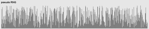
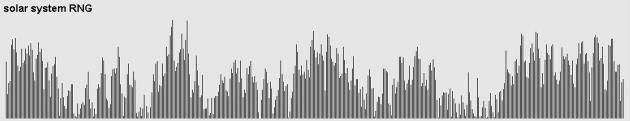
Elementary variables are not enough random to be used
inside program algorithms. In the next step the program calculates the
secondary variables using more or less complex mathematical equations where
elementary variables are applied. This approach enables application of a great
number of different random generator formulas. In order to produce the needed
interval of values the division with the remainder is used. On Figure 04 there
are presented two graphs of random numbers: computational (Visual Basic RND
function) and physical (Solar System).
figure
04
5. Program description
For the described purpose I developed an experimental
program which enables one to study and analyze the whole system and to
demonstrate the results that are generated during it’s run. The results of the
program are images, a color harmonized abstract with no form definition or any
kind of similarity to the real world. The program uses a typical pragmatic
approach where selected object are posted in a selected position of the plane.
The program run is not absolutely autonomous because it allows some
intervention from the outside especially on setting different process
parameters. The drawing algorithm is of course independent of any human input.
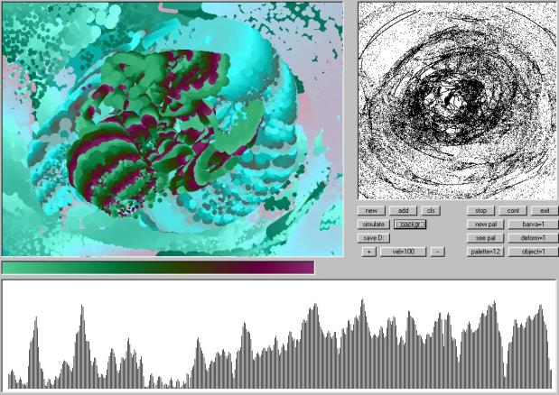
The program is running in an infinite loop commanded from the outside using
command buttons. On Figure 05 the user graphic interface with a working area is
presented.
figure
05
The program is object oriented Visual Basic executable
and consist of some sections performing different tasks:
-
An initialization section where main
program parameters are defined: a starting position of the planets, circular
motion velocity and starting command values (color palette, coloring algorithm,
deformation type, drawing object type and others),
-
A simulation section where the solar
system motion is simulated,
-
A calculation section where all
needed elementary variables are calculated (distances between planets and
distances between actual drawing point and planets),
-
The main section with a pulsing
spiral curve which calls all other section participating in the drawing process
-
A deformation section, object
drawing section, coloring algorithm section, graph drawing section etc,
-
A command section with command
buttons actions.
The user graphics interface is designed for resolution
1024 x 768. On the upper left part of the screen there is a main operating window
where images are generated. The same window is used to present the momentary
set of coloring palettes and to simulate the solar system’s movement in a scale
that enables us to observe all planets revolving on their orbits. The upper
right window is designed to track the movement of the drawing point. The lower
part of the screen is dedicated to the random number graph presentation. In the
middle left there is visible the coloring palette in use. The command section
is positioned in the middle right with command buttons (start new cycle, add
new cycle, stop processing, continue processing, set velocity, change of color
algorithm, set coloring algorithm type, set deformation type, set object type,
set new palette package, make palette visible, change palette in use, clear
screen, exit program etc).
The coloring algorithm is the hearth of every
generative program with the task to create images. The pixel or the object
color is the result of a more or less complex mathematical calculus called a
coloring algorithm or coloring formulas. Not only computational methods are
applied and some authors use decomposition of another image to define the color
sequence if a new image [9]. To define the color of image elements I used two
types of coloring algorithms: index based approach and direct coloring
formulas. Index based coloring formulas return a floating-point number which
acts as an index into a color map or color palette and the color is not
specified directly. The color map could be created inside the program or could
be imported from the outside. Direct coloring formulas calculate the color
(three RGB components) for each pixel or object directly [10]. The set of
coloring palettes which is created in the beginning of every program cycle
could be redesigned at any moment during the program run and is saved in a
three-dimensional matrix.
The program draws objects on a two-dimensional plane,
for example circles, ellipses, squares, lines, curves and other geometrical
forms and also forms which are created randomly. The position of the object is
defined by a dynamic drawing point described above. Starting the program is
possible to select a drawing object, deformation type, type of coloring
algorithm, the coloring palette and a velocity of the solar system which has an
important influence on a random number generator. During the program’s
execution all these parameters could be changed interactively using command
buttons.
6.
Program results
The results of the experiments realized so far are
absolutely abstract images more or less centrally oriented. The colors are
harmonized if the process is autonomous or the manual color selection is done
during a momentary suspension of the program. Changing color parameters when
the program is running causes interesting images to form but they are color
not-harmonized. Depending on the selection of a good deformational style the
image loses its self-similarity elements which appear in a different position.
The best results are created leaving constant starting color parameters but
changing the deformation and object type. Alternating from-center and to-center
drawing process causes additional chaotic effects into the final results. The
described concept is close to the idea of perfect abstract creations which
don’t resemble any object from the real world. In Figure 06 some examples of
images are presented.
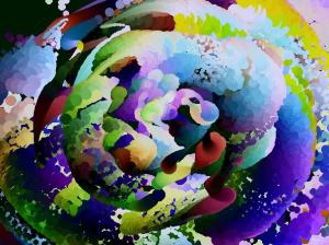
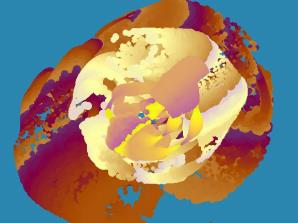
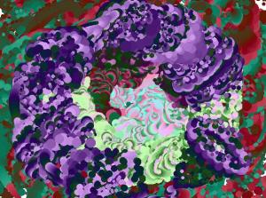
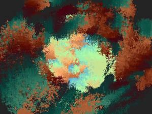
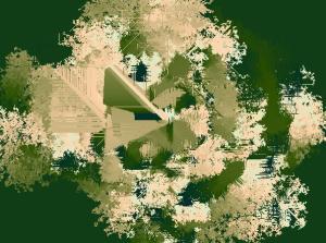
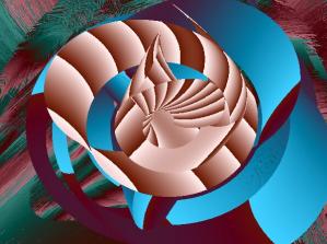
figure
06
7.
Conclusion
For the experiment presented in this
paper I used a limited number of variables which are produced inside the solar
system. The first results have become a serious challenge to develop this idea
furtehr to obtain more complex and interesting images. The number of parameter
variants used in the program (type of deformation, type of object, color
palette creation) could be larger to obtain more different and unpredictable
results. In the program only one system of a dynamic drawing point is used.
Instead of the spiral curve a more complex movement could be applied, for
example a combination of two, three or more mathematical graphs: circle,
ellipse, spiral, cycloid, polynomial function or others. The set of drawing
objects could be supplemented with new types especially those with irregular
forms. There is an immense number of possibilities to combine formulas to draw
irregular objects pixel by pixel and to respect defined conditions of a
previously drawn element. Analyzing examples of generated images and having in
mind all not yet used possibilities I can conclude that the described idea to
use the solar system as a physical random number generator could be a very
productive and creative approach in the area of developing a generative
algorithm to create artworks.
References
[1] Paul Trow, Chaos and the Solar System,
http://www.geocities.com/paul_bt@sbcglobal.net/essays/ChaosandSolarSystem4.htm?20062
[2] Bill Arnett, An Overview of the Solar System,
http://www.nineplanets.org/overview.html
[3] Calvin J. Hamilton, Views of the Solar System, http://www.solarviews.com
[4] John Walker, Solar System Live, http://www.formilab.ch/solar/
[5] University of Geneva, Random Numbers, http://www.randomnumbers.info
[6] University of Utah, Random Number Generators, http://www.math.utah.edu
[7] Benjamin Jun, The Intel Random Number Generator,
http://www.cryptography.com/resources/whitepapers/IntelRNG.pdf
[8] Robert Davies, True Random Number Generator,
http://www.robertnz.net/hwrng.htm
[9] Bogdan Soban, Generating Artworks Using Previous Created Image as
Coloring Palette, GA 2005, Conference Proceeding
[10] Chaospro documentation, Coloring Formulas, http://www.chaospro.de