Evolving Street Plans from
Shops and Shoppers
C.P. Mottram, BA, MSc.
Bartlett School of Architecture, UCL, London,UK.
Abstract
Using an agent based model
where the agents use vision as their main method of navigation combined with a
simple economic model we attempt to derive simple cities.
Within the cities the "shops" and the agent
"shoppers" develop a topology, as shops survive either through visits
from the agents or are destroyed by the agents "stealing" their
goods, eventually the shape of the city settles to some optimum form where all
the shops make money and the shoppers endlessly wander.
1.
Introduction
Architecturally
we might consider the various town plans as aesthetic entities which derive
their aesthetic from both the economic background and the nature of the people
who inhabit the city.
Here we are
going to use agents to try and simulate aspects pertaining to both of these, we
shall try to alter the economic landscape and the nature of the agents and see
what happens.
The two kinds
of agents are going to be called “shops” which stay still and “shoppers” who
move.
We hope to
evolve solutions from the location of the “shops” which have the appearance of
street plans that might be found in a real city.
We want the
street plans themselves to be sustainable, that they conduct the movement of
the “shoppers” in such a way as to optimize the income for the sedentary
“shops”, that a diverse range of shops is maintained over an appreciable time,
that an agent should always be able to find the correct shop with a minimum
number of steps.
These are
fairly difficult criteria so many of our solutions are unstable. We shall look
mainly at the areas where we have found stable solutions and consider, if
possible, the implications and character of these “solutions”, how to
strengthen and weaken the solutions by alterations to the model.
We will also
try to guess at the existence of other solutions, where the simulation is
moving from its current state to something which more closely resembles
reality. From this we might try and derive which are the most important
characteristics which should be added to the simulation.
1.1 The Basic Economic Model
This economic
simulation takes two simple elements, a shopper who moves and a shop which
stays still.
The shopper
moves among the shops “purchasing” items, each time a shopper makes a purchase,
a number is added to the “shops” balance and the “shopper” agent is reset to
try and purchase some thing else.
If the
“shopper” agent cannot find a shop selling the item it seeks then the shopper
agent attempts to become a “shop” agent.
The shops are
“taxed” at each iteration, ie a small amount is subtracted from their balance, if
the balance gets to zero the shop agent becomes a shopper.
Thus if there
are too few shoppers the less successful shops will become shoppers. If there
are lots of shoppers but not enough shops, some of the shoppers will become
shops.
We wish to use
this natural balance to manage the self regulation of this agent economy.
This balances
“supply” shops and “demand” shoppers which can be a problem in economic models.
This allows us
to concentrate on the shape or topology of the city, to drive it towards various
optima. These optima might be thought of what is the city “best for”, is the
overall revenue the best criteria, or maybe the stability or perhaps the
shortest travel distance for the purchase of any particular item, these are all
points of view, say the city government, the shops’ or the agents’. Other views
might be considered as we seek to define different optima. The total sum of
these “best for” scenarios we might define as the “aesthetic” of the city, or the “beauty” of the city if you
like, as the city in the real world will combine many different features within
a single whole.
Perhaps it
might be possible at this moment to clarify that the agents’ purchases are not
subdivided into groceries, insurance etc. but remain as abstract concepts, we
could imagine that these are the kind of purchases necessary for the shopping
agent to live and that the probability of an agent seeking out a particular
kind of shop has a critical bearing on the form of the city, the tension then
between supply and demand provides one of the major dynamics for the city as a
whole.
To summarise
the basic factors which alter the economic profile of the simulation are:-
Shop
income,
Based on
number of visits of agents to front of shop, shop balance is increased by the
shop price.
Rent
Based on the
number of agents passing by, (relative attractiveness of location).
If a shop is
in a busy area while not doing much business it is probably unsuitable for the
area and will go out of business.
Poll tax
Decrements balance every
iteration, so shops need visitors to keep solvent.
Thief tax
Agents approaching shops
from behind decrement shop balance to
encourage back
to back shops systems.
Dynamic
tax.
The Rent and
the Poll tax can be incremented or decremented automatically by a fixed amount
depending on either the proportion of shops to people or the average shop life
of the shops.
The metrics
for considering the viability of the system are
1. Average
shop life,
2. Number of
steps between purchases,
3. Total tax
income generated
These are all
recorded in a spreadsheet
Clarity of
road plan, agents trails are marked by dark lines, if lots of agents walk the
same way the trail becomes progressively darker, and shops are less likely to
be placed on the trail.
We can also
make the program save a bitmap of the city at repeated intervals, this allows
us to make animated avi’s or “movie” files, these can be useful to watch the
development of the city over many 1000s of iterations. This makes it possible
to find those areas which are stable over long periods and those which are
constantly changing.
Initially we
started these simulations where price and item were separate, the same “item”
might be sold at different locations by different shops at different prices.
This was meant
to uncover detail to do with different pricing levels in different
neighbourhoods, unfortunately it was impossible to “see” this on the maps,
without radically changing the visualisation. So the maps presented have only a
single factor, the price, effectively the price and the item become the same
thing. Where red is expensive and blue is cheap.
1.2 The Agent Model
The agents’
“world” is a simple two dimensional field which can be coloured to provide
areas of relative attractiveness, the agent “sees” the world using a simple
sampling method using three vectors. One directly ahead, and two at a variable
angle to this to the left and to the right. The agent chooses its path either
by choosing the longest line or by choosing the most attractive shop, which will
be chosen by a variety of criteria such as price, item and distance, the
distance viewed is weighted by the colour of the ground, where black is zero
and white is one.
The variable
angle is randomly set at each iteration dependent on the distance “seen” by the
agent, if the distance is very short the angle is set wider until if the
distance is very short the angle is set to provide 180 degree vision, remember
this is a sample so the agent will not always choose the longest possible line.
1.2.1 Ways of changing gaols.
We have
experimented with various methods of choosing where an agent goes next having
made a purchase. There are two parts to this, firstly how is the new “taste” or
preference chosen and secondly how does one get there. We’ve made some attempts
also to ask, “what would the agent want if it knew how far away it was or how
expensive it was?” we shall discuss this in the “how does one get there”
section.
1.2.1.1 How to choose a taste.
weighted
random v multiple needs
The original
method was to use a weighted random, where the current taste was used as an
input to the next taste. So the next taste was defined as the current taste
plus or minus a random number to the size of the current taste.
This meant
that small current taste would lead to the next taste being at most twice the
current taste and at lowest zero which we pad up to one. If however the current
taste is high we have an equal chance of the next taste being anything. This
was meant to provide a weighted random, where expensive purchases occur rarely,
and that cheaper purchases occur in proximity to each other and possibly in
progression.
We also tried
a “normal random” where new taste is assigned in a purely random fashion.
The multiple
need method assumes an agent has a range of needs which occur at different time
intervals, so you might want a snack every couple of hours and maybe buy a new
TV every three to five years and want to go to the supermarket every week, to
this end we have an agent continually review its “need state”, and whenever a
need goes critical this becomes the agent current taste, and the agent starts
searching for the new need, once this is satisfied, it resumes the quest it had
before, or deals with any other need which has become critical. As a further
complexity the satisfaction of one need can be set to lead to a suppression of
adjacent needs, also the visibility of
a taste will accentuate a need, thus if an agent can see something and
its close, the critical need is accentuated to make the agent more likely to purchase
this item.
The speed at
which these different needs become critical can be randomly set over a profile,
so no two agents will have the same order of purchasing, this we speculate
might be termed a “personality” as defined by a purchasing profile.
Personality
could be defined as a predilection for a certain range of purchases, thus for
an individual agent this might be the probability distribution of the taste
change at each new purchase.
Variations of
random distribution, or a specific profile working within the multiple need
set.
1.2.1.2. How does one get there?
Either the
agent wanders aimlessly following the longest line and its taste vectors or we
can build a model of memory for the agent, so it can remember where it
purchased something.
There are two
ways we have done this, one is to give each agent a map of all the places it
has visited, the second is to allow the agents to access a common memory map of
the whole city.
We have tried
both, the computer memory needs of the first method, led to some problems and
we also felt it was slightly unrealistic, as when we as people are lost we can
always ask somebody or look at a map, to be only able to access one memory is
not typical human behaviour! Unless you’re a visitor to a city, who speaks none
of the language of the city and can’t read maps, and has done no preparation.
We thought this was probably an unusual situation, though there might be reason
to examine this more closely in the future, especially when agents get a “home”
which would include a home area or neighbourhood, where they would behave
differently than in the rest of the city.
So most of the
time we allowed the agent full knowledge of the city, to allow it to make a
decision based on its current location related to is current need set. At this
point the metric between distance, price and how closely an item matched a need
became very important. The cost of distance becomes crucial to avoid all the
agents choosing the same shop ( the cheapest ), even then we might expect the
best shop to become hidden behind shops of the same item but a higher price, in
practise this didn’t happen much, so the cost of distance became central and
crucial once knowledge was added to the system.
Knowledge,
partial and complete, cost of distance v specialization of purchases.(
purchaser discrimination)
1.2.1 When does a shopper become a shop.
There are some
strategic goals here, in that we wish to build village settlements, so shops
should be built where and when they are needed, the need then is provided by
the shoppers, so the weight of “need” in any particular area is balanced by the
shops available
Generally we
use a combination of the following factors to decide this.
When it’s
walked more than a certain many steps without finding a shop or when the average
number of steps per purchase becomes too great.
When it finds
an opportunity, sufficient space.
When it’s made
a particular number of purchases.
We can set the
proportion of shops to people to limit the number of shops, alternatively we
can use the average shop life to increase taxes when the numbers get too high
or when the proportion of shops gets to high, and similarly the taxes get
decremented when the numbers of shops is low. This control tends to be useful
in getting an idea of what the optimum tax or proportion of shops should be for
a given configuration.
Generally
different methods lead can lead to different patterns initially, though on
longer runs these tend to disappear as the old adage of location takes control,
and the surviving shops from whichever method assume similar patterns.
1.2.2 Rules for shop placement.
A shop will be
placed at a location relative to the “shopper” location not more than three
times the size of the shop at the location, firstly that is not already
occupied by another shop, and secondly that has the lowest count of shopper
trace steps ( where the background is lighter). This will mean that shops
generally are placed beside the places where shoppers are walking. This also
tends to reinforce the routes created by the shoppers.
2. Interim Results
Initially we
will show results using different methods of choosing the next item. We can
compare results from agents which are using the multi-need model to agents
using a simple weighted random. This will be done with the tax set at two
levels as this accentuates the differences between the results.
The main
measure we will use from the data gathered is the average shop balance, where a
city is successful the average balance will be high and rising quickly. This
data is gathered every 100 iterations, we can use this in conjunction with the
mean price of the shops and the deviation from this mean which will give us a
measure of diversity.
We can see
easily enough that for the low tax situation in Figs 1 and 2 the maps
are fairly similar, they are fairly maze like in that few long straight vistas
have opened up, in Figs
3
and 4, a medium tax
example, we can see the differences have appeared. The multi-need version has
become a kind of grid and the weighted random one has broader curves, taking on
a simpler pattern. In Fig
5
a high tax sample using the weighted random, we now have something which looks
like the multi-need model.
This gives us
a good idea of the critical function of the shopper behaviour on the survival
of the shops when stress, as in higher taxes, are applied to the model.
We used 3000
agents in these simulations, setting a shop size to be 10, and where the actual
size of the city was about 808 x 377 pixels, the proportion of shops to
shoppers was set to be 0.3, though in none of the runs was this number reached,
we were in fact packing them to maximum sustainable density. Low tax was 0.1
high tax was set to 1.0 and very high tax was set to 2.0. A shop is given an
initial balance of a 100, so if a shop was unvisited in the high tax situation
it would survive 100 iterations.
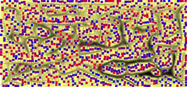
Fig 1. Low tax with
simple weighted random method of choosing target
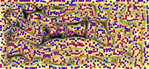
Fig 2. Low tax with
multi need decisions.
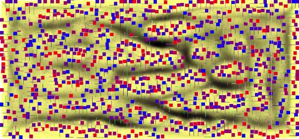
Fig 3. High tax with
simple weighted random
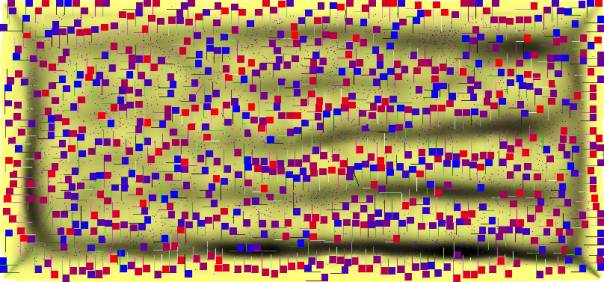
Fig 4. High tax with
multi-need decision making
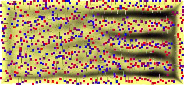
Fig 5. Very high tax
with simple weighted random
It can be seen
in Fig 5 that the dark horizontal bands starting on the right fade out as they
move to the left, this indicates that we are on the edge of stability, the
following graph indicate the average balances of the five.
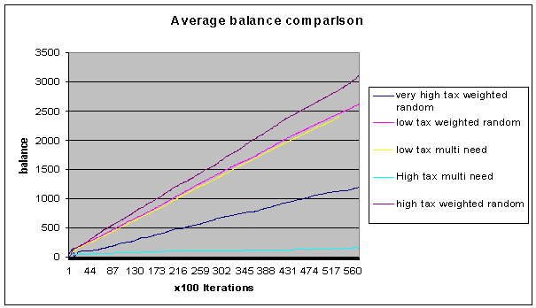
Fig 6. Average
balance of shops compared
We can see
here that the high tax multi need never really gets off the ground we might
assume that this is an example where we haven’t found a reasonable solution.
The shops haven’t found a configuration which works with the shoppers’ method
of choosing their target!
The very
interesting and slightly unbelievable thing about this graph is that the high
tax weighted random has a higher average balance than the low tax and the very
high tax, this would seem to suggest that the tax can within certain ranges
force the map into a more efficient pattern which can negate the effect of
higher taxes. In other words, shops which were “in the way”, preventing
shoppers from reaching their destinations are no longer able to survive and the
actual “efficiency of the system” is improved. Remember too that this effect is
due to a flat rate or “poll tax” also note that as the tax is raised again the
average balance is reduced, so this suggests a curve which reaches an optimum
and then goes down again. To investigate the shape of this curve we would have
to plot points on it by rerunning the experiment with a finer range of
different tax levels.
The average
balance is calculated by adding together the balances of all the shops and
dividing it by the total number of shops and shoppers together, this gets
around possibilities of false high readings where we might have very few shops
and lots of shoppers. 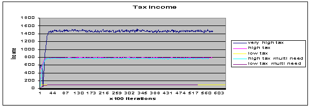
Fig 7.This shows the
actual tax deducted in the scenarios described above.
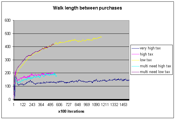
Fig 8. Steps between
purchases compared.
Here we show
the average number of steps between purchases, this if you like is the cost to
the shopper, you can see that for the shopper the very high tax reduces
distance between purchases.
Its also best
for the city as it gives the highest tax revenue, unfortunately its not the
best for the shops, the highest average balance was found in the high tax
bracket.
Also when we
count the actual number of purchases over the first 53300 iterations the very
high tax comes first with 6693 followed by the high tax weighted need at 5649,
followed by the multi need high tax at 4195.
Both the low
tax situations gave the lowest number of purchases with the weighted need on
3109 and the multi need low tax getting the least number of purchases at 3027.
Shoppers have
to find shops for purchases to occur so possibly this is the best indicator
of the navigability of the city by very
stupid shoppers.
3. Discussion
We have shown
that various parameters can alter the visual look and the economic wealth of
the city. From the view of the shopper, the shop and the city different
parameters can sometimes work in unison.
In our
simulation we have shown that a critical facility such as a tax can have a
function to improve the quality of the city, by improving the shape of the city
to improve life for the agents the shops and for the city, there can be a
consensual optima which is dependent on the subtle alteration of simple
parameters.
Why are we
doing this? Internet shopping might make high street shopping redundant. Thence
our need, in cities, is for areas for socializing which have different economic
driving forces, which will be different from the ones presented here. Perhaps
we will have to define an economics of social intercourse to replace the
economics of material exchange?
This is closer
to theories of knowledge and the way information is disseminated, which has a
rich semantic, its graph theories, theories of social networks etc.
In another
guise we might become historians rather than planners, guessing something of
the nature of the people and their economics by the kind of street plans they
leave behind.
The other
thing we like to think of is how intelligent the cities are as a means of
optimising the stresses we impose through the simulation. Can all these little
decisions made by the agents add up to something which is really useful? Is the
summation of multiple aesthetics really an ideal of beauty or are we entering
the economic basement of the lowest common denominator, finding the solutions
with the most winners and discarding the losers. To this end we have to
consider that the more complex agents did not produce solutions, the city
configuration could not be optimised on their behaviour. These were agents who
were endlessly distracted, forever changing gaols as their various diverse
needs came to the fore. Its interesting to see that they still managed to make
similar numbers of purchases within the same number of steps as Fig 8. shows. So
even though no stable configuration appeared the economy was still working at
almost the same rate as the weighted random samples. It is possible that some
other behavioural key would make this simulation work to produce a world where
the shops survived as well.
4. Further Work
We haven’t
presented the effect of knowledge on the behavioural patterns within this
paper, This is mainly due to a shortage of space. Our findings were that the
cost of distance was critical to avoiding simple monopolistic outcomes, indeed
to create a homogenous multi centre city, where the shoppers always know the
location of where to find the “best deal” becomes very difficult. There is an
instability in the concept of total knowledge which means that the centres are
dynamic and frequently move around.
To this end we
thought that we might try and stabilise this by reducing the agents’ knowledge
to a neighbourhood, within which they might have perfect knowledge, but
outside, and when they wish to purchase some thing which does not reside in
their neighbourhood, they will have very little knowledge. This is work which
we are in the process of conceiving
Another
dynamic we thought to introduce is that associated with the daily flows from
home to work and back again, for this would add a third agent representation,
that of the home with the associated need for space and quiet. This has a
simple economic, which would site home in areas where the shopper count is low,
its “value” as a home with some restorative effect combined with its closeness
to shops to reduce travel costs, might
need some zonal statistics, to establish areas of low v high activity, these
zonal statistics would also enable us to establish where the actual centres of
activity were in our city, and find out if there is shopper movement from
centre to centre, or whether all movement is from centre to periphery and back
again.
To this end we
also want to run the simulation where shoppers will only purchase within a
limited range, then if there are two groups, each only purchasing within a
range, will the groups separate spatially, and what will the pattern of the
interface?
We will also
be analyzing the results produced so far in an attempt to see if the
simulations show features which can be reliably observed in real cities.