Deepland, a Travel through
many Dimensions
M.-P. Corcuff
GRIEF, Ecole Nationale Supérieure d’Architecture de
Bretagne, Rennes, France.
COSTEL, LETG UMR 6554 CNRS, Université Rennes 2, Rennes,
France.
e-mail:
m-p.c@wanadoo.fr
5.1
Abstract
After a few recalls about the topological definition of dimension and
some of the topics that have to do with this crucial issue, this paper focuses
on the search for regular polytopes by folding, on complete, incomplete and
recursive tiling, and on recursive folds, in order to travel, not only from
dimension to dimension, but through dimensions.
5.2
Introduction: Dimension
Let’s recall
first the inductive topological definition of dimension. Our space is
three-dimensional (3D) because we are not forbidden to go from any part of it
towards another by any point (0D), nor by any line[1]
(1D), but we may be “cut” from another part of space by a surface (2D). Any
space is nD when it is cut by a (n-1)D space, but not by a (n-2) or lower
dimension space. This definition does not apply only to common sense space, but
is valid for any continuum, for example the “space” of colours [3].
We consider an
“empirical continuum” defined by our perceptive system (including our
kinaesthetic sense), and not a mathematical continuum, nor the physical
phenomenon, which may be not continuous, or which may have another structure
than our perception of it: “space” is 3D for us human beings, relatively to our
visual and tactile senses, essentially, plus our “sense of displacement”, or
kinaesthetic sense, i. e. the muscular perception of movement which permits to
link different visual or tactile perceptions with each other. But it does not
mean that “space”, as a physical object, is 3D: actually, physicists consider
much more dimensions than three in their latest models, though we’ll never be
able to directly perceive it.
Being
inductive, this definition implies that dimension is an integer number, which
matches our intuition. Being topological, it applies without having to define a
metrics on space. Topology considers objects which can be stretched and
deformed as we wish (without tearing them though): a square is the same as a
circle for topology, it is simply a closed line. But this definition is
coherent with our more usual use of dimension for space with a metrics, i. e.
the coordinates (any point of a 3D space needs 3 coordinates to be located, 1
or 2 are not enough, 4 are too much), or the way measures grow when the linear
size (1D) grows: area (2D) as a power 2, volume (3D) as a power 3 of the linear
measure.
This
definition applies also to parts of space, to objects or figures of a space. As
a corollary of the topological definition of dimension, the limit (boundary,
border, edge) of a part of nD space is (n-1)D: a segment (1D) has got two
points (0D) as its border; the border of a disc (2D) is a circle (1D), that of
a square (2D) is made of four segments (1D), that we can also consider as one
folded line; the border of a sphere (as a 3D volume) is a sphere (as a 2D
surface); that of a cube (3D) is made of six squares (2D) that we may consider
as one folded surface. We see there an important paradox of this issue of dimension:
though a segment has got a border (constituted of two points), a circle, which
is also a 1D object has got no border… In the same way, the surface of a sphere
(2D) has got no border: a part of a space of less than 3 dimensions can be
finite (bounded) without being limited! However, we cannot conceive a volume
without a border, unless it is the whole space itself…
The paradox of
a bounded unlimited surface is easy to conceive, as the surface of the earth is
roughly a sphere, and we know well that if we travel on it ahead of ourselves
for a long enough time, we’ll come back to our starting point… But we are 3D
beings, and though we are in a great part tied to the surface of the earth, we
can also see it from 3D space, and observe that it has got no border
because it is curved, and curved in such a way that it closes upon itself. We
even can ourselves make a closed surface, for example by folding an adequately
cut sheet of paper (a rough approximation of a part of a plane) into a cube
(the surface of it): we can fold it because we are 3D people… For a
surface to be curved, or folded, we see that it must be immersed in a space of higher dimension, namely for a
surface 3D space. But how a volume could be curved or folded , as we cannot
conceive of a 4D space in which it would be immersed?
The inverse of
the above corollary is that any unlimited nD object defines (i. e. is the
border of) at least one (n+1)D object: on a plane, an infinite line defines two
half planes; a circle defines a disc and the remnant of the plane with a
circular hole; on a sphere, a great circle (the equivalent of a straight line
on the sphere) defines two hemispheres; on a torus, a circle defines a surface
which we can assimilate to a finite cylinder. Similarly, in 3D space, an infinite
plane defines two “half-spaces”, the surface of a sphere defines a solid sphere
and the remnant of space with a spherical hole, etc.
We human
beings are 3D individuals living in a 3D space. This is so obvious that we
don’t daily question it. More than one hundred years ago, some authors, the
most famous of them being Edwin Abbott Abbott with his novel Flatland: A
Romance of Many Dimensions By A Square [1], undertook to make their readers
more open-minded to their 3D condition by imagining, mainly, 2D beings living
in a 2D space: to be aware of their possibilities and limitations makes us more
conscious of our own possibilities and limitations, and of our own means of
representation of 1D, 2D and 3D objects, and even 4D objects, which are not
more inconceivable, after all, than 3D objects are for 2D beings (which we, as
“superior” beings, can observe with some condescension). This comparison is
indeed efficient and throws light on evidences and paradoxes of our 3D fate.
Thomas F. Banchoff [2], among others, has prolonged this endeavour: this paper
owns a lot to his work.
A way to go
from nD to (n+1)D is folding. In the search for regular polytopes, we’ll
focus on that way to go from one dimension to another, but we’ll also try to
not only jump from one dimension to another, but to go through
dimensions, to explore that unknown world that lies between 1D and 2D, between
2D and 3D…
5.3
1. Regular polytopes and
folding
Regular
polytopes (polygons, polyhedra, etc.) are a favourite item of mathematicians to
characterize spaces of any dimension, as soon as a metrics is defined on those
spaces. It is not generally question of a regular “polytope” in 1D; it is
however obvious that we can extend the definition of a regular polytope on a
line, by observing that a segment answers to this definition, i. e. an object
with the maximum of symmetry possible in its space. That the segment is
actually the only object possible in its space makes its status of
regular polytope too trivial to be generally mentioned. Going from dimension to
dimension by the way of regular polytopes seems very simple. The most often
referred to is to start from a point, then to get a segment by
moving the point in one direction, and to go from there to a square by
moving the segment in the second direction , then to a cube by moving
the square in the third direction; if you consider our 3D space it is the end
of the travel, but it is easy to imagine that in 4D space there is a 4th
direction available, which allows to go from the cube to a hypercube by
“moving” the cube in that 4th direction; and so on…
Actually there
is another even simpler way to accomplish this travel. At each step, instead of
moving the previous polytope in some direction, you can add a vertex (a point)
to the previous polytope; then the succession of polytopes becomes: point,
segment, equilateral triangle, tetrahedron, etc… In the 4th
dimension we can imagine adding a vertex to the tetrahedron in the same way
that we add one to the triangle in the 3rd to obtain what may be
called a pentatope (since it has got 5 vertices, and five hyperfaces, or
“cells”). Those simplest polytopes, which are constituted by (n+1) vertices
defining triangles in any nD space are called simplexes.
So we have, in
any dimension, at least, a “cube” (which we call a square in 2D), and a
“simplex”. To find other ones, one way is to consider the “duals”; the dual of
a polytope is the polytope obtained by placing the vertices of the new polytope
in the centre of the faces of the previous one: for example, in 3D, the dual of
the tetrahedron is itself a tetrahedron, but the dual of the cube provides a
new polyhedron: the octahedron. Actually, it can be demonstrated that any
simplex is “self-dual”, and that there exists a dual polytope of the “cube”,
distinct from it, in any dimension higher than 2. So there are at least 3
regular polytopes in any dimension…
Actually, in
any dimension higher than 4 those 3 regular polytopes are indeed the only ones.
But in 2D, they are infinitely many regular polytopes (polygons), and they are
all self-dual; in 3D there are 5 polytopes (polyhedra), one is self-dual (the
tetrahedron) and the two other pairs are dual of each other (resp. the cube and
the octahedron; and the dodecahedron and the icosahedron); and in 4D there are
6 (the simplex, which is self-dual, two pairs of dual polytopes, and another
one which is self-dual)… This shows the complexity of dimension, behind its
seemingly simple and boring enumeration:
1, 2, 3, 4,…
Among the many
ways to define and produce regular polytopes, one, which goes from dimension to
dimension, is that of folding. Any child knows how to make a cube starting from
a sheet of paper dexterously cut into connected squares. Actually, we don’t
miraculously create a volume (3D) starting from a sheet of paper (roughly 2D)…
We only produce a surface that encloses such a volume, the “skin” of a
cube. But as we have seen before, a closed surface defines at least one volume.
Trying to fold regular polytopes around a regular polytope (all of the same
kind) in any dimension is a way to find all the regular polytopes in the space
of higher dimension[2]. The
restraints we have are to respect some symmetry, and to let enough looseness to
be able to fold.
Let’s start in
2D, and let’s try first to place regular polygons around another one, by
patching them edge to edge. You can place 3 triangles around a triangle, and by
folding them up, you obtain the tetrahedron (Fig. 1.a). You can place 4 squares
around a square and by folding, you obtain an open cube that you close with a 6th
square (Fig. 1.b). You can place 5 pentagons around a pentagon, and by folding
those, you obtain half of a dodecahedron, that you can close by another
symmetric half, rotated (Fig. 1.c). Now if you place hexagons around an
hexagon, there is no place left to fold them (as they tile 2D space, as we’ll
see further). If you try with heptagons, etc, there is even superposition, so
you cannot fold them.
Now, let’s
return to the square and the triangle and let’s try to add other squares (resp.
triangles), touching now by the vertices. With the square, as soon as you add
those 4 new squares, the plane is filled and you cannot fold them out. But with
the triangle, there are two new possibilities: you can add three new triangles,
and by folding, you obtain an open octahedron, which you close with a last
triangle (Fig. 1.d). Or you can add 6 new triangles (2 at each vertex) and you
obtain the half of an icosahedron, which you complete with another half, by
rotating it, as for the dodecahedron (Fig. 1.e). Now if you try to add 3 new
triangles, you fill up the plane, and you cannot fold them out.
Figure 1 shows
the start of the folding patterns (above), and the Schlegel diagrams (below) of
the regular polygons: Schlegel diagrams are actually usual perspectives, but
where the camera is placed very near from the object, and with a very great
focal angle, so that the front face embraces all the other ones:
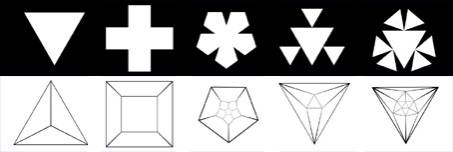
Figure 1 a b c d e
Now let’s
return back to 1D. Instead of playing with paper, scissors and tape, a child
can play with sticks or matches (all these games are dangerous anyway). We can
place two segments around one, and that is all we can do, by the way, as
segments have two vertices, but have no “edges” in 1D space. We can fold them
easily around their extremities (we may want to tie them, but loosely), and
they kindly rejoin each other to make a triangle. Now, to make other polygons,
we can fold them less, and let some space for a 4th segment, to get
a quadrilateral. But here we encounter a problem that did not exist in going
from 2D to 3D, which is that we do not compulsorily obtain a square, or that
this square collapses easily upon itself… Actually, all polygons made of more
than 3 segments collapse, where any convex polyhedron is uncollapsable: here is
one the mysteries of dimension… Anyway, let’s try to arrange our quadrilateral
into a fair square, and let’s resume our game. We see that we can add as many
segments as we want and thus obtain all the (regular, if we are careful)
polygons.
Going from 3D
to 4D, we see that we can place 4 tetrahedra around one, and we have only to
fold them in 4D space to obtain the 4-simplex (Fig 2.a)[3].
And we can place 6 cubes around one, and fold them to obtain an open hypercube,
which we’ll close with an 8th cube to obtain the hypercube (Fig.
2.b). We can also place 8 octahedra around one, this will produce a polytope
made of 24 octahedra, which is called 24-cell (Fig. 2.d,e,f). And we can put 20
dodeacahedra around one, to get a more complicated polytope, the 120-cell (Fig.
2.c).
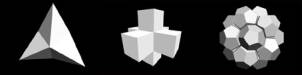
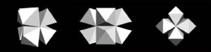
Figure 2 a b c d e f
Now, can we
place polyhedra, not only against faces of another one, but between these,
against edges, as we have done against vertices of polygons. It is only
possible if we start from the tetrahedron. We can place 4 more tetrahedra this
way to get the 16-cell (Fig. 3.a,b,c). And there is even some place left (not
much, but enough…), to put one more tetrahedron, and this leads to the most
complex 4D polytope, the 600-cell (Fig. 3.d,e,f).
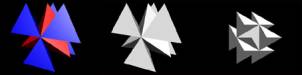
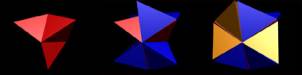
Figure 3 a b c d e f
5.4
2 Complete, incomplete, and
recursive Tilings
Trying to find
ways to fold out polygons into polyhedra, we have encountered situations where
the plane was filled, namely with equilateral triangles (with 12 of them around
one), with squares (with 8 of them around one), with hexagons (with 6 of them
around one), and that’s all (higher polygons overlaid). Those situations
correspond to the possible regular tilings of the plane.
On a line, any
segment defines a “tiling”. On a circle, though, the segment (which is an arc)
must be a divider of the circumference. On the plane, the equilateral triangle
(Fig. 4.a), the square (Fig. 4.b), and the hexagon (Fig. 4.c) define tilings:
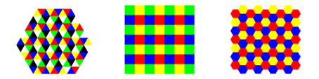
Figure 4 a b c
On the sphere,
tiling is even more restricted than on the circle: only the regular polyhedra
define a tiling, or tessellation, of the sphere:
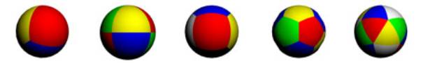
Figure 5
Let’s return
to planar tiling, and let’s examine those patterns, according to some
regularities. For example, let’s compare the distribution of the vertices and
of the centres of the polygons: we see that for the squares they are the same,
but that for the triangles and the hexagons they swap: we could say, referring
to the vocabulary used for polyhedra, that the square (orthogonal) tiling is
self-dual, but that the triangular and the hexagonal ones are duals of each
other.
This duality
may be expressed in another way. If we apply the principle of the distance map
[3] to the three distributions of centres, we see that the Voronoï diagrams we
get are those so-called dual tilings.
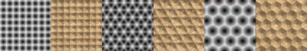
Figure 6
We can also
consider tiling as a cellular automaton, and launch a growth process. Usually
CA consider cells as pixels on an orthogonal grid. But we can consider any
tiling polygon as well. Starting with a polygon, we apply the rule that we’ll
add all the same polygons we can that touch the previous ones at each step. We
obtain different patterns according to the neighbourhood chosen to apply the
rule: as in a CA we can consider only the edges (Fig. 7.a,c), or the edges and
the vertices (Fig. 7.b,d). For the hexagon, there is no difference (Fig. 7.e):
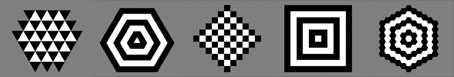
Figure 7 a b c d e
We see that
this growing process leads to a pattern similar to the starting polygon, only
in one case: the square, and with the second rule.
Those polygons
are the only ones that actually tile the plane. But why not try the same growth
process with a pentagon? It leads to an incomplete tiling:
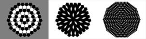
Figure 8
This
experiment with the pentagon gives us the idea to try other incomplete tilings,
even with the polygons that tile the plane. It is produced by adding a new rule
to the previous one: we’ll not add a polygon if it touches more than one
of the previous generation. These incomplete tilings with the triangle (Fig.
9), the square (Fig. 10), the hexagon (Fig. 11), and the pentagon (Fig. 12) provide
interesting patterns:
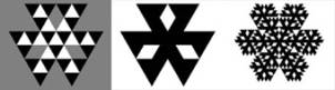
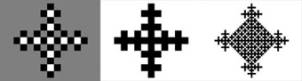
Figure 9 Figure 10
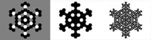
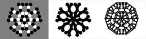
Figure 11 Figure 12
Now, returning
to our first patterns, we notice that the square produces a square, but that
the hexagon does not produce an hexagon, and the equilateral triangle neither.
That has to do with self-similarity: we know that the square is self-similar
(i. e., that it can be filled up with reduced copies of itself), but that the
hexagon is not. But we thought that the equilateral triangle was self-similar
too, didn’t we? Well, it is, but upon the condition that we accept to change
the orientation of one the reduced copies…
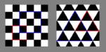
Figure 13
Self-similarity
is another way of defining dimension. Let’s observe the patterns we got before
in this way. In 1D, when we have added two segments around one, we have
obtained a segment filled up with 3 reduced copies of itself, 3
times smaller. In 2D, the square is filled up with 9 copies of itself,
reduced by 3; the alternative pattern of the equilateral triangle (where
we permit a change of orientation) shows a triangle filled up with 4
triangles 2 times smaller. In 3D, the only self-similar polyhedron, the
cube, is filled with 27 cubes 3 times smaller. The dimension
(self-similarity dimension, which in those cases matches the topological one)
is obtained by dividing the logarithm of the number of copies by the logarithm
of the number by which those copies are reduced: for the segment, we get log 2
/ log 2 = 1; for the square: log 9 / log 3 = log 32 / log 3 =
2 log 3 / log 3 = 2; for the triangle: log 4 / log 2 = log 22
/ log 2 = 2 log 2 / log 2 = 2; for the cube: log 27 / log 3 = log 33
/ log 3 = 3 log 3 / log 3 = 3: which is coherent with their topological
dimension.
So we can
consider another way of tiling, which is recursive tiling. We know that
the triangle and the square fill the plane so their recursive tiling is not
very satisfying. But we can do it with a triangle from which we have removed
the middle reduced one, and we obtain the well known Sierpinski gasket:
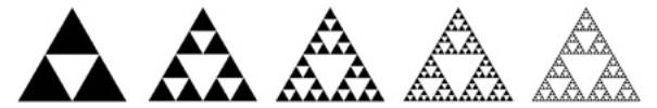
Figure 14
But we have
seen that the pentagonal tiling did not fill the plane. So we can apply the
recursive tiling to it:
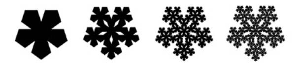
Figure 15
Now, in 3D,
only the cube tiles (or “tessellates”) space, and it is also the only one
polyhedron that is self-similar. The tetrahedron could be a good candidate for
self-similarity. After all, it is the equivalent of the equilateral triangle
which is self-similar. Unhappily, when you stack tetrahedra in the way you
stack triangles in the plane, the hole in the middle is not in the form of a
tetrahedron, or any number of tetrahedra, but is in the form of an octahedron!
Anyway that
does not prevent us to try recursive 3D tiling (or tessellation) with those 4
tetrahedra:
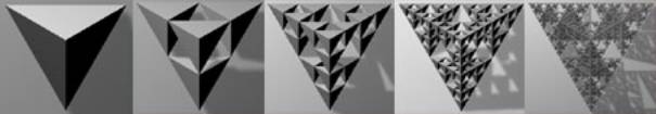
Figure 16
The stacks of
polyhedra we did to find the 4D polytopes may also lead to recursive
tessellations. Let’s take the one that lead to the 24-cell. It is enclosed in a
bigger octahedron. So we can repeat the multiplication of octahedra on this
first stack:
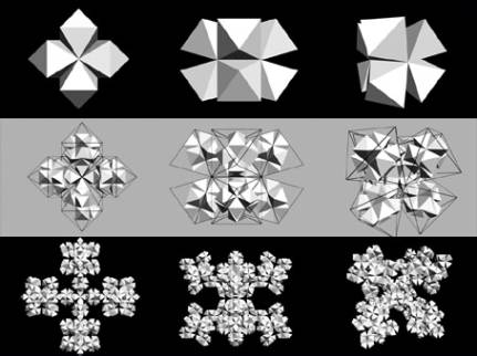
Figure 17
Incomplete
recursive tilings and tessellations allow us to reach paradoxical objects
because their self-similar dimension is not an integer. For example, if we
apply the definition mentioned above to the Sierpinski gasket (Fig. 14), which
is made of 3 copies of itself, reduced by 2, we get: log 3 / log 2 = 1.58…; for
the recursive pentagonal tiling (Fig. 15), we find 1.86… With the recursive
tetrahedral tiling (Figure 16), we encounter a new paradox: d= log 4 / log 2 =
2. This figure is equivalent to a surface! Indeed, if you rotate the
tetrahedron above and move it down, you see that you actually end up with a
plane. If you add a fifth tetrahedron below, you obtain a fractal dimension of
log 5 / log 2 = 2.32…:
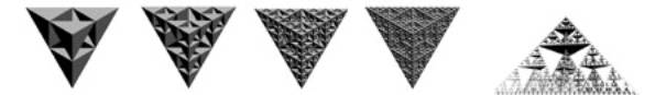
Figure 18
Those
recursive incomplete tilings lessen the dimension of the object from which they
start: from 2D to somewhere between 1 and 2; from 3D to somewhere between 2 and
3. We’ll see with recursive folds processes that increase the dimension.
5.5
3. Recursive folds
Our complacent
child is now bored with cutting paper and taping it, and he crumples the sheet
of paper to throw it in the wastebasket (we have removed the matches, though…).
Now that is interesting because in this way he has produced some sort of ball,
which is actually nearer from a real 3D form than the skins of polyhedra he obtained
with much effort before. Well, if we are fastidious, we’ll not accept that this
“ball” is a real 3D volume, but we must accept that it is a good approximations
of it. Examining a crumpled sheet of paper, we see that it is not only folded,
but that the folds are re-folded, and re-folded, and that it is actually a
recursive fold.
The most known
recursive fold of a line is the von Koch curve, of self-similar dimension log 4
/ log 3 = 1.26…:
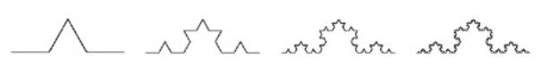
Figure 19
Recursive
folds are ways to obtain figures which are of a dimension between 1 and 2, but
can we actually travel all the way from 1D to 2D? Yes, because there are
extreme cases where the self-similar dimension is equal to 2[4];
We can change the angle in the von Koch construction (Fig. 20.a: 15° d=1.012…
b: 30° d=1.05… c: 45° d=1.13… d: 60° d=1.26… e: 75° d=1.50… f: 90° d=2), to get
a curve that fills a part of the plane:
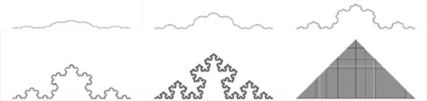
Figure 20 a b c d e f
There are even
such recursive folds that fill a 3D volume. The Hilbert curve fills a cube:
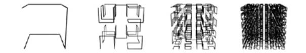
Figure 21
The von Koch
construction reminds us of the way we have folded a line to make a triangle. We
can try another recursive fold based on the square:
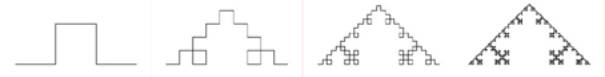
Figure 22
You can fold a
line any way. But folding a plane is more difficult, because you must do folds
in alternate senses. So we’ll admit to call folds operations that are not
actually folds, but which consist of pulling vertices of a plane outside the
plane. We can for example try to adapt the previous folds we made from a line
to a triangular or square surface:
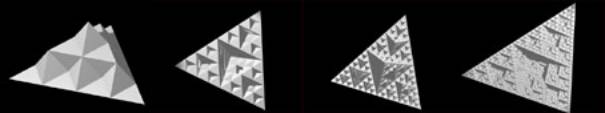
Figure 23
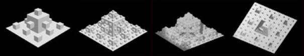
Figure 24
Note that in
the case of the triangular folded surface, the “peaks” touch on the outside, so
the complexity is better seen from below. The fractal dimension of this
“surface” is log 6 / log 2 = 2.58…, that of the square one is log 13 / log 3 =
2.33…
5.6
Conclusion
Folding is a
very good way to creativity, as proves the Japanese art of origami or the
experiment in “folding as a morphogenetic process in architectural design”
proposed by Sophia Vyzoviti [4]. Tilings
have also been much exploited, for example in islamic art. The aim of
this paper was just to propose some leads to see forms, even such familiar
forms as regular polygons and polyhedra, in a different way, to see them as
part of a transforming process [5]. Many of these leads could be pursued much
farther. Those experiments make us also more aware of what is dimension, of
what link dimensions with each other, and of what could lie between them.
5.7
References
[1] Abbott,
Edwin Abbott, Flatland: A Romance of Many Dimensions By A Square, first
published by Seeley & Co, London, 1884
[2] Banchoff,
Thomas F., Beyond the Third Dimension: Geometry, Computer Graphics and
Higher Dimensions, Scientific American Library, 1990
[3] Corcuff,
Marie-Pascale, “Generative processes and the question of space”, GA 2005
proceedings
[4] Soddu,
Celestino, “Gencities and visionary worlds”, GA 2005 proceedings
[5] Vyzoviti,
Sophia, Folding Architecture: Spatial, Structural and Organizational
Diagrams, BIS Publishers, 2003